
Three different questions: reaching a destination in fewer steps, finding the cheapest route, and connecting every point at minimum total cost. One graph helps us distinguish the objectives.
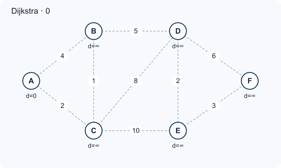
A graph consists of vertices V and edges E. Our graph is simple, undirected and connected: each edge can be traversed both ways. It has 6 vertices and 9 edges. Edge numbers are costs, not drawing lengths. Neighbours are processed alphabetically; equal-weight edges are ordered by name. A path joins vertices; a cycle returns to its start without repeating other vertices. A tree is connected and has no cycles.
A–B: 4 A–C: 2 B–C: 1 B–D: 5 C–D: 8 C–E: 10 D–E: 2 D–F: 6 E–F: 3
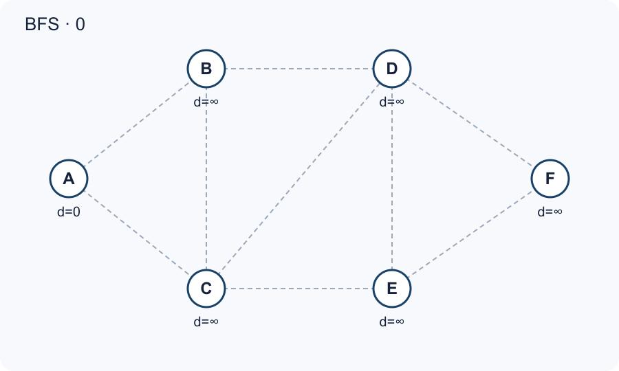
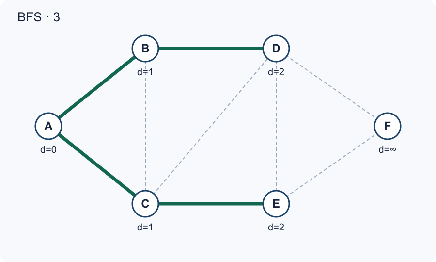
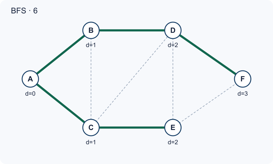
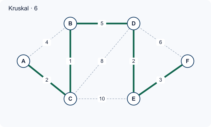
Solid green lines: selected edges or current predecessors; dashed grey lines: other edges. BFS omits weights. Intermediate Dijkstra predecessors can change. ∞ means no distance has yet been found.
1. BFS: the fewest steps
Breadth-first search ignores weights: each edge counts as one step. Starting at A, we find the minimum number of edges to every reachable vertex. A FIFO queue removes the oldest entry first.
Set d(A)=0 and enqueue A. Remove the first vertex u; for each undiscovered neighbour v, set d(v)=d(u)+1, record u as predecessor and enqueue v. Mark vertices when enqueuing, not when removing, to avoid duplicates. Continue until the queue is empty.
| Step | Vertex / edge | Queue / settled set / cost | Distances in order A, B, C, D, E, F |
|---|---|---|---|
| 0 | — | [A] | 0, ∞, ∞, ∞, ∞, ∞ |
| 1 | A | [B, C] | 0, 1, 1, ∞, ∞, ∞ |
| 2 | B | [C, D] | 0, 1, 1, 2, ∞, ∞ |
| 3 | C | [D, E] | 0, 1, 1, 2, 2, ∞ |
| 4 | D | [E, F] | 0, 1, 1, 2, 2, 3 |
| 5 | E | [F] | 0, 1, 1, 2, 2, 3 |
| 6 | F | [] | 0, 1, 1, 2, 2, 3 |
After A the queue is [B,C]. B discovers D; C discovers E but does not overwrite D. D discovers F. A–B–D–F uses 3 edges. A–C–E–F also uses 3: an optimal path need not be unique. The first path costs 15, so fewer steps need not mean lower cost.
Why it works
- Invariant: the queue is ordered by nondecreasing distance. While level k is processed, new vertices join the end at level k+1.
- Base case: A correctly has level 0. Inductive step: if all vertices up to level k have correct distances, each newly discovered neighbour of a level-k vertex is reachable in k+1 edges.
- It cannot have a shorter distance: its predecessor on a shorter path would have been processed at an earlier level and would already have discovered it. Thus the first assigned distance is minimal. Predecessors reconstruct a shortest path.
With adjacency lists each vertex is enqueued once and each edge inspected twice: O(|V|+|E|) time and O(|V|) auxiliary memory, excluding the graph. In a disconnected graph, only the source component is visited.
Princeton · Algorithms, 4th Edition — BFS
2. Dijkstra: the cheapest path
Weights now matter and must be nonnegative. d(v) is the best path cost found so far, initially infinity except d(A)=0. S contains vertices whose distances are settled.
Choose the vertex u outside S with smallest d(u) and add it to S. For each neighbour v outside S, relax the edge: d(v) ← min(d(v), d(u)+w(u,v)). Update the predecessor whenever the value improves. If the minimum is infinity, remaining vertices are unreachable.
| Step | Vertex / edge | Queue / settled set / cost | Distances in order A, B, C, D, E, F |
|---|---|---|---|
| 0 | — | {} | 0, ∞, ∞, ∞, ∞, ∞ |
| 1 | A | {A} | 0, 4, 2, ∞, ∞, ∞ |
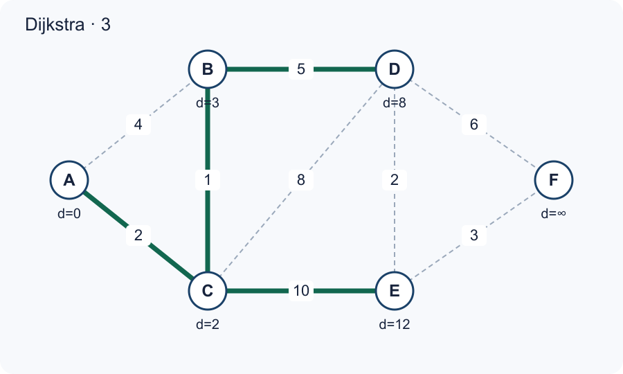
| 2 | C | {A, C} | 0, 3, 2, 10, 12, ∞ |
| 3 | B | {A, C, B} | 0, 3, 2, 8, 12, ∞ |
| 4 | D | {A, C, B, D} | 0, 3, 2, 8, 10, 14 |
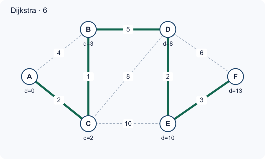
| 5 | E | {A, C, B, D, E} | 0, 3, 2, 8, 10, 13 |
| 6 | F | {A, C, B, D, E, F} | 0, 3, 2, 8, 10, 13 |
After A: B=4, C=2. C improves B to 3 and proposes D=10, E=12. B improves D to 8. D improves E to 10 and proposes F=14. E improves F to 13. The optimal A–C–B–D–E–F costs 2+1+5+2+3=13 but uses 5 edges, more than BFS.
Why it works
- Every finite estimate is the cost of an actual discovered path, so it never underestimates the optimum. Assume all settled distances in S are correct.
- Suppose the selected minimum u had a cheaper path. Let y be its first vertex outside S and x its predecessor in S. When x was processed, relaxation gave y an estimate no greater than the cost of this path prefix.
- Nonnegative remaining weights mean the prefix costs no more than the entire path to u. Hence d(y) would be smaller than d(u), contradicting the minimum choice. The distance to u is settled correctly; induction proves all extractions correct.
Adjacency lists and a binary heap with decrease-key give O((|V|+|E|) log |V|) time and O(|V|) auxiliary memory. Scanning vertices to find each minimum takes O(|V|²+|E|). Negative weights invalidate the proof: with directed edges A→B=2, A→C=5, C→B=−10, B is settled at 2 although its optimum is −5.
Princeton · Algorithms, 4th Edition — Dijkstra
3. Kruskal: connecting everything cheaply
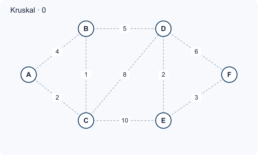
We seek a network joining all vertices with minimum total edge weight, not a route from A to F. This is a minimum spanning tree (MST). A tree with 6 vertices has exactly 5 edges.
Sort edges by increasing weight. Initially each vertex is its own component. Accept an edge only when it joins different components; otherwise it creates a cycle. Union-Find checks and merges components. Stop after |V|−1 accepted edges.
| Step | Vertex / edge | Queue / settled set / cost | Kruskal |
|---|---|---|---|
| 0 | — | 0 | — |
| 1 | BC (1) | 1 | Selected |
| 2 | AC (2) | 3 | Selected |
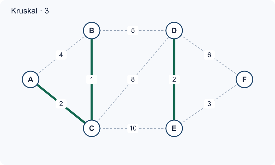
| 3 | DE (2) | 5 | Selected |
| 4 | EF (3) | 8 | Selected |
| 5 | AB (4) | 8 | Rejected: cycle |
| 6 | BD (5) | 13 | Selected |
First edges: BC(1), AC(2), DE(2), EF(3), AB(4), BD(5). Reject AB because A and B are already joined through C: it closes A–C–B–A. BD joins {A,B,C} and {D,E,F}. Total: 1+2+2+3+5=13. DF(6), CD(8), CE(10) need not be processed.
Why it works: an exchange argument
- Invariant: some MST T contains all edges already selected in F. Initially F is empty. Let e be the next accepted edge, joining different components of F.
- If e belongs to T, nothing changes. Otherwise adding e creates one cycle. That cycle contains an edge f leaving the component of one endpoint of e; f is not in F. Also w(f)≥w(e): a lighter edge crossing that component would have been processed earlier and merged the components.
- Replace f with e. The result remains a tree and its cost cannot increase. Since T was minimal, the new tree is also minimal and contains F together with e. The invariant is preserved. After |V|−1 accepted edges, the constructed tree is an MST.
Sorting takes O(|E| log |E|). Union-Find with path compression and union by rank takes O(|E| α(|V|)) overall, almost linear. Memory is O(|V|+|E|), including sorted edges. Negative weights are allowed. A disconnected graph yields a minimum spanning forest rather than one tree.
Princeton · Algorithms, 4th Edition — Kruskal
Here Dijkstra and Kruskal both yield 13 and the same edges, but this is a coincidence. In the triangle AB=2, AC=2, BC=1, the shortest-path tree from A uses AB and AC (total 4). An MST uses BC and one weight-2 edge (total 3). In that tree one route from A costs 3 instead of 2. Different objectives produce different answers.