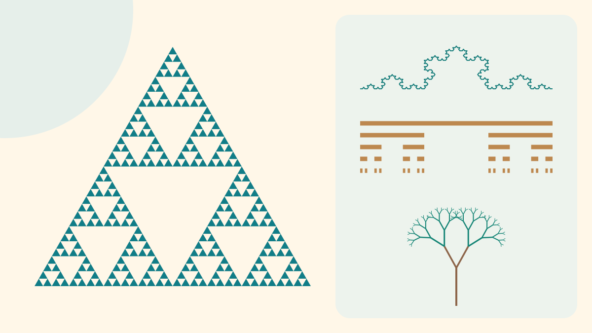
Can a triangle lose almost all its area without disappearing? Can a curve grow longer and longer while staying inside a small region? Can a few instructions generate a complex landscape? Fractals let us investigate these surprising questions with examples we can check.

We start with pencil-and-paper constructions, gradually introduce powers and logarithms, then reach computer-generated images. You do not need complex numbers for the first constructions: the more advanced part is explained separately.
1. What is a fractal?
A magnified square still looks square, but looking along one edge does not repeatedly reveal a whole square. In many fractal constructions, smaller and smaller parts reproduce the organisation of the whole: this is self-similarity. It is exact in the Sierpiński triangle, whereas in a real tree it may only be approximate or statistical.
Benoît Mandelbrot introduced the word fractal in 1975, drawing on the Latin fractus, broken. Being irregular is not enough to make something a fractal, and not all fractals are perfect copies of themselves or have non-integer dimension. We will study precise models with explicitly stated rules. (B. Mandelbrot · Fractal Roughness (WPI)).
Distinguish the mathematical limiting object from its image. The former is defined by a potentially infinite process; the latter stops after a finite number of stages and pixels. Increasing detail does not mean reaching infinity.
2. Sierpiński: less area, more triangles
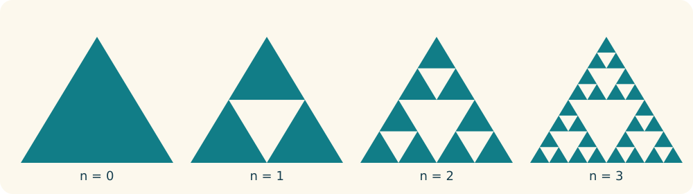
Draw a filled equilateral triangle. Join the midpoints of its sides to form four equal triangles. Remove the middle triangle and repeat on the three remaining ones. Call the initial triangle n = 0: each new level triples the number of triangles and halves their side length.
Why is the area factor 3/4? Three triangles remain, each with half the previous side and therefore one quarter of the previous area: 3 × 1/4 = 3/4. After three levels there are 27 triangles with sides 1/8 of the original side. Their combined area is 27/64 of the initial area.
To convert the ratio to a percentage, explicitly multiply by 100%: (27/64) × 100% = 42.1875%. At level 5 there are 243 triangles, yet only (3/4)⁵ × 100% ≈ 23.7305% of the initial area remains. The piece count increases while total area decreases. In the limit the area tends to zero without the set becoming empty.
Nₙ = 3ⁿ
lₙ / l₀ = (1/2)ⁿ
Aₙ / A₀ = 3ⁿ × (1/2)²ⁿ = (3/4)ⁿ
A% = (3/4)ⁿ × 100%| Level n | Elements at level n | Remaining area |
|---|---|---|
| 0 | 1 | 100% |
| 1 | 3 | 75% |
| 2 | 9 | 56.25% |
| 3 | 27 | 42.1875% |
| 4 | 81 | 31.640625% |
| 5 | 243 | 23.730469% |
| 6 | 729 | 17.797852% |
3. Cantor: removing without emptying everything
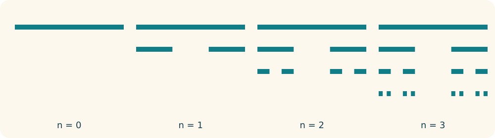
Start with a unit segment. Remove its middle third, leaving two segments of length 1/3. Repeat on both: four segments of length 1/9 remain. After n steps there are 2ⁿ intervals, each of length 3⁻ⁿ.
The total remaining length is 2ⁿ × 3⁻ⁿ = (2/3)ⁿ. At level 4 this is 16/81; as a percentage, (16/81) × 100% ≈ 19.7531%. Each row in the laboratory represents a different time: do not add the lengths of different rows.
The limiting total length is zero, but many points remain: for example, endpoints 0 and 1 are never removed. Having zero length is not the same as containing no points. The limiting model has dimension about 0.63093: it is thinner than a segment, not merely a short segment.
Nₙ = 2ⁿ
lₙ / l₀ = (1/3)ⁿ
Lₙ / L₀ = (2/3)ⁿ
L% = (2/3)ⁿ × 100%
4. Koch: infinite length, finite area
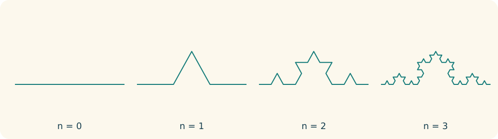
Divide a segment into three equal parts. Replace the middle third with the other two sides of an outward equilateral triangle. One segment has become four, each one third as long. Repeat the operation on all new segments.
The length factor is 4 × 1/3 = 4/3. Starting with 9 cm, after three steps the length is 9 × (4/3)³ = 64/3 cm ≈ 21.3333 cm. Individual segments become shorter, but their number grows enough to make total length increase without bound.
Starting from the three sides of an equilateral triangle produces the Koch snowflake. With initial side 10 cm, the starting perimeter is 30 cm; level 3 has 192 segments and perimeter 30 × (4/3)³ ≈ 71.1111 cm. The enclosed area, however, tends to 8/5 of the initial triangle’s area. Infinite perimeter and finite area describe the limit, not a finite drawing.
For the area formula, sum the small areas added: the first increment is A₀/3 and each subsequent increment is 4/9 of its predecessor. The geometric series gives Aₙ/A₀ = 8/5 − (3/5)(4/9)ⁿ. The fractal dimension refers to the snowflake boundary; the filled region inside has dimension 2.
Nₙ = 4ⁿ; Lₙ = L₀ × (4/3)ⁿ

Koch curve and snowflake
Pₙ = P₀ × (4/3)ⁿ
Aₙ / A₀ = 8/5 − (3/5)(4/9)ⁿ
A∞ / A₀ = 8/5 = 1.6
5. Dimension: how does a structure occupy space?
Two half-sized copies reconstruct a segment: 2 × (1/2)ᴰ = 1 gives D = 1. A square needs four half-side copies: 4 × (1/2)ᴰ = 1 gives D = 2. A cube needs eight copies and D = 3.
For self-similar models with suitably separated copies, use N × rᴰ = 1, where N is the number of copies and r is their length ratio. Taking logarithms gives D = log(N)/log(1/r). Any logarithm base works, provided it is the same in numerator and denominator.
For Sierpiński, N = 3 and r = 1/2 give D ≈ 1.58496. For Koch, N = 4 and r = 1/3 give D ≈ 1.26186. Do not automatically apply this formula to a photograph or arbitrary branching pattern: overlaps and different assumptions require further checks. The laboratory displays the dimension of the limit, not that of the small filled triangles at a finite level.
D = log(N) / log(1/r)
| Limiting model | Copies N | Ratio r | Dimension D |
|---|---|---|---|
| Cantor | 2 | 1/3 | 0.63093 |
| Koch | 4 | 1/3 | 1.26186 |
| Sierpiński | 3 | 1/2 | 1.584963 |
6. More examples: carpets and sponges
The Sierpiński carpet starts from a square split into nine small squares. Remove the middle one and repeat on the eight remaining pieces. After n steps there are 8ⁿ squares with total area (8/9)ⁿ of the original. The limiting dimension is log(8)/log(3) ≈ 1.89279.
The Menger sponge is three-dimensional. Split a cube into 27 smaller cubes, then remove the centre cube and the six face-centre cubes, retaining 20. After n steps its volume is (20/27)ⁿ of the initial volume and its limiting dimension is log(20)/log(3) ≈ 2.72683.
Compare the rules: 3 half-scale copies in the triangle, 8 one-third-scale copies in the carpet, and 20 one-third-scale copies in the sponge. Complexity comes from repeating a short rule, not from a very long description. These last two models are article examples, not extra laboratory modes.
7. Building a tree with recursion
Draw a trunk. Two shorter, angled branches grow from its tip. Repeat at each new tip. With ratio r = 0.65 and trunk length 1, successive generation lengths are 1; 0.65; 0.4225; 0.274625; and so on.
Level 0 has one segment. At level 4 the drawing contains 1 + 2 + 4 + 8 + 16 = 31 segments, including 16 terminal branches. Here earlier generations remain in the count, unlike the count of final triangles in Sierpiński.
Changing angle and ratio in the laboratory produces narrow trees, wide trees or overlapping branches. The resemblance to a natural tree is a geometric model, not a botanical simulation. We do not assign dimension using the simple formula log(2)/log(1/r), because overlaps can change its interpretation.
Nₙ = 1 + 2 + 4 + … + 2ⁿ = 2ⁿ⁺¹ − 1
Nₜ = 2ⁿ
lₙ / l₀ = rⁿ
8. Iterating a formula: complex numbers first
Iteration means repeatedly applying the same rule to the previous result. For instance, z → z² + 1 starting from 0 produces 0, 1, 2, 5, 26. Each result becomes the next step’s starting value.
Mandelbrot and Julia pictures use the complex plane. A number z = x + iy corresponds to point (x,y), with i² = −1. Parameter c = a + ib is another point. No special library is needed: separating real and imaginary parts translates the formula into two operations on real numbers.
An orbit is the sequence z₀, z₁, z₂, … . It is a calculation history, not a planet’s motion. Some orbits stay bounded; others grow without bound. This distinction organises the pictures.
zₙ₊₁ = zₙ² + c
(x+iy)² + (a+ib) = (x²−y²+a) + i(2xy+b)
xₙ₊₁ = xₙ² − yₙ² + a
yₙ₊₁ = 2xₙyₙ + b
9. Mandelbrot: a map of parameters
For the Mandelbrot set, fix z₀ = 0 and vary parameter c between pixels. Parameters whose orbit stays bounded belong to the set. Each pixel asks: what happens to 0 for this c?
Simple real examples: c = 0 keeps the orbit at 0; c = −1 alternates between 0 and −1; c = −2 gives 0, −2, 2, 2, … . For c = 1, instead, we obtain 0, 1, 2, 5, … . At step 3 the modulus exceeds 2 and escape is established. The inequality must be strict: reaching exactly 2 is not enough.
A computer tests only finitely many iterations. If a point does not escape within 160 steps, this test alone cannot show it never will. In the laboratory, black means no escape observed within the chosen budget; colours distinguish escape times. Increase the budget, select a point and zoom: you are exploring numerical detail, not proving membership for every point. (R. Devaney · Mandelbrot Set Explorer (Boston University)).
10. Julia: changing the starting point
For Julia, exchange what stays fixed and what varies: choose one parameter c and test many initial points z₀. The filled Julia set consists of initial points with bounded orbits; the Julia set itself is its boundary.
The case c = 0 is especially revealing: z is repeatedly squared. If |z₀| < 1 its modulus tends to 0; if |z₀| > 1 it grows; if |z₀| = 1 it stays 1. The filled set is therefore the unit disk and its boundary is a circle. Not every parameter produces a jagged boundary.
Then try c = −1 or c = −0.8 + 0.156i: very different forms emerge. The escape criterion used is |z| > max(2, |c|), safe even when |c| exceeds 2. Again, testing is finite and dark points are non-escaping candidates unless we have an additional proof, as for c = 0. (Boston University · Filled Julia sets).
11. Is nature really fractal?
Romanesco broccoli repeats small cones resembling the whole head; a fern’s leaflets echo the organisation of its frond. Tree branches and river networks show branching hierarchies. They are excellent examples of multiscale organisation without being exact geometric copies.
A coastline looks more intricate when measured with a shorter ruler: previously ignored inlets enter the count. The result depends on measurement scale and method, not only on a supposed single number called length. Statistical models can describe this dependence over a range of scales. (B. Mandelbrot · Coastlines and fractal dimension (PNAS, 1975)).
Clouds, mountain profiles and lightning can show multiscale complexity; blood vessels and airways have branching structures. Yet a striking photograph does not by itself establish a fractal law: measurement needs data, specified scales and a checked model. Cells, grains, molecules and physical processes interrupt repetition.
12. Applications: why this geometry matters
Procedural graphics combine details at different scales to generate terrain, clouds and textures. A few parameters control an image rather than drawing each detail. Fractal noise is not the Sierpiński triangle, but shares the idea of organising several scales. (K. Perlin · Procedural Textures (NYU)).
In telecommunications, some antennas use fractal geometries to obtain compact structures or multiband behaviour. Shape alone does not guarantee better performance: materials, frequencies and electromagnetic design also matter. This is a specific engineering application, not a magical property of every fractal drawing. (Fractal Antenna Systems · Technical overview).
Image analysis can compare complexity and branching; art and design use repetition and changes of scale. In box counting, overlay grids of spacing ε and count cells touching the shape. The slope of log N(ε) against log(1/ε) can estimate dimension only across suitable scales. A few pixels or grids do not yield a universal value.
13. Guided laboratory experiments
1. Sierpiński: start at level 0 and move one step at a time. Before pressing Next, predict the triangle count and remaining area. Check level 5 and compare 243 triangles with approximately 23.73% remaining area.
2. Cantor: examine level 4, count the 16 intervals and check their combined length 16/81. 3. Koch: switch from open curve to snowflake, comparing perimeter growth with the area ratio approaching 1.6.
4. Tree: choose level 4 and ratio 0.65, then change the angle. The count stays 31 while the shape changes. 5. Mandelbrot: choose c = 1, then c = −1; compare their orbit tables. 6. Julia: choose c = 0, observe the disk and test initial points with modulus below and above 1.
Calculations run in the browser without sending parameters to the server. Level limits keep constructions usable on phones; complex images can be interrupted. Animation displays one level at a time and tables support numerical comparison. A stopping condition is essential in programming: without one, recursion would keep calling itself.
14. Try it yourself
Make a prediction or calculation before opening an answer. Solutions are hidden: reveal only the one you want to check.
1. How much Sierpiński area remains at level 4?
Show the explained solution
There are 3⁴ = 81 triangles. Each has side 1/16 and area 1/256 of the original. Combined area: 81/256 = (3/4)⁴. Convert to a percentage: (81/256) × 100% = 31.640625%.
2. A Koch segment starts at 27 cm. What is its length at level 3?
Show the explained solution
Each level multiplies length by 4/3: L₃ = 27 × (4/3)³ = 27 × 64/27 = 64 cm. There are 4³ = 64 segments, each 1 cm long.
3. Why can Cantor have zero length without being empty?
Show the explained solution
The remaining length is (2/3)ⁿ and tends to zero. Endpoints 0 and 1 remain at every stage and belong to the limit. That alone rules out an empty limiting set.
4. Does a tree at level 6 have 64 or 127 segments?
Show the explained solution
64 is the number of terminal branches, 2⁶. The drawing also retains trunk and earlier generations: 1 + 2 + 4 + 8 + 16 + 32 + 64 = 127 = 2⁷ − 1 segments in all.
5. Is a black pixel after 400 iterations certainly in the Mandelbrot set?
Show the explained solution
No: we only know that the test has observed no escape within 400 steps. Escape may occur later. Certain membership requires another argument, such as the fixed point 0 when c = 0.
6. For Julia with c = 0, what happens to z₀ = 1/2 and z₀ = 2?
Show the explained solution
In the first case 1/2 → 1/4 → 1/16 → 1/256 → … tends to 0. In the second 2 → 4 → 16 → 256 → … escapes. The filled set is the disk |z₀| ≤ 1; its boundary is the circle |z₀| = 1.