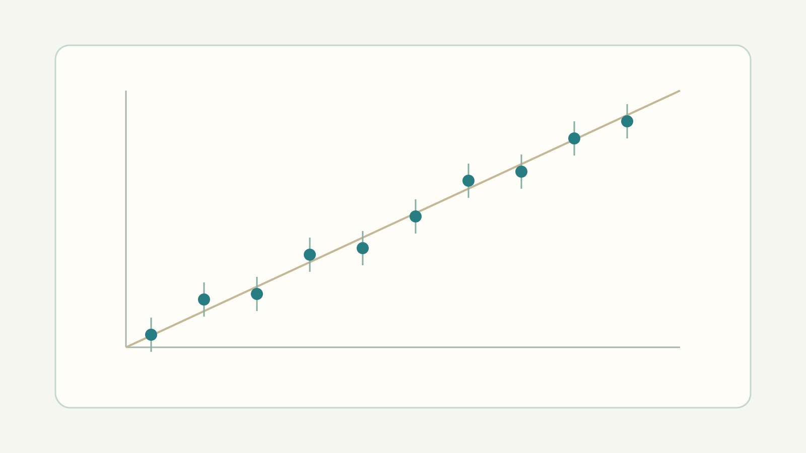
Correct arithmetic is not enough. Check data and forecasts over time, measure errors and compare changes without using the future.

1. Three different checks
Arithmetic check: do the same data and rules produce the same numbers? Data check: do rows describe the correct matches, goals and times? Predictive validation: do probabilities issued before events describe many subsequent outcomes well? Passing the first check does not pass the others. A data fingerprint proves identity, not truth.
The two examples permit arithmetic checking, not an honest accuracy or profitability measurement. We use explicitly invented examples to learn the tools, not as results achieved by the real model.
2. Audit the archive before formulas
Keep match ID, competition, teams, home/away role, UTC kickoff, regulation-time score, completed status and availability time. Deduplicate by ID. Check GF and GS refer to the studied team; compare a sample with the original source. Do not turn missing data into zero goals.
Freeze data, version and parameters before forecasting. Corrected data require a new version: never silently rewrite the original forecast after seeing the outcome. We have aggregates for 537 matches, not every row; record this limitation.
3. Separate past and future
Training estimates the model using only the available past. Validation compares choices in a later period. Final testing evaluates the already fixed choice once on a last period never used for decisions. Exact dates and duration depend on the archive; do not choose them after seeing results.
past data → forecast next block → observe outcomes → move forward → repeat
This is rolling-origin evaluation: forecast first, observe later. At each step recompute competition means using only admissible past data. Randomly mixing future and past matches, using final standings or odds unavailable at forecast time leaks future information.
4. Compare against something simple
A first simple alternative uses only competition μ_H and μ_A with the same Poisson distribution, without team factors. A second uses unweighted team averages on the same eligible matches. These are comparison baselines. Use identical events and periods for all: complexity does not imply improvement.
5. Record a complete forecast
| Quantity | Meaning |
|---|---|
| ID, UTC, cutoff | Event identity and frozen times |
| version, h, m, window | Rules and parameters fixed beforehand |
| λ_H, λ_A, P1, PX, P2 | Full forecast, not just favourite |
| G_H, G_A, y | Outcome added only afterwards |
Do not save only the most likely outcome. (0.40, 0.35, 0.25) and (0.98, 0.01, 0.01) both choose 1 but express very different confidence. Counting correct top choices loses this information. Add the observed outcome later without changing saved probabilities.
6. Measure error: Brier step by step
Invented example: the outcome is X, a draw. In order (1,X,2), the observation vector is y=(0,1,0): one for the occurred category, zero elsewhere. Forecast U: p=(0.50,0.25,0.25). Forecast V: p=(0.25,0.50,0.25). Subtract the observation from each probability, square and add. Here we sum all three categories without dividing by two.
Brier=Σ(p_c−y_c)²
U: (0.50−0)²+(0.25−1)²+(0.25−0)²
   =0.25+0.5625+0.0625=0.875
V: (0.25−0)²+(0.50−1)²+(0.25−0)²
   =0.0625+0.25+0.0625=0.375
Lower is better; this convention ranges from 0 to 2. V is better on this case, not necessarily overall. Across n matches add the n scores and divide by n. It is not a win percentage and does not alone describe calibration.
7. Penalise misplaced confidence
Log loss uses the probability assigned to the outcome that occurred. Apply ln, the natural logarithm, and change sign to get non-negative loss. Lower is better. In the draw example U assigned 0.25 and V assigned 0.50.
loss=−ln(p_actual)
U: −ln(0.25)≈1.386294
V: −ln(0.50)≈0.693147
Assigning zero probability to an event that occurs gives infinite loss. If software guards rounding with a minimum threshold, document it; it must not hide catastrophic forecasts. Compare mean loss over many matches alongside Brier, counts and other checks.
8. Does a 70% forecast behave like one?
Calibration compares probabilities with observed frequencies. For the same event, group similar forecasts; compare group mean probability with the fraction of events occurring. Invented example: 100 forecasts at 70%, 68 occurrences. Frequency=68/100=0.68; 0.68×100%=68%. Difference: 68%−70%=−2 percentage points.
Two numbers are not enough: show group counts and sampling uncertainty. Five events tell little. Lower Brier alone does not prove better calibration; discrimination between situations also matters. Do not confuse percentage points with percentage change.
9. Change a parameter, not chase an outcome
| Match | m | λ_H ≈ | λ_A ≈ | P1 × 100% |
|---|---|---|---|---|
| Shakhtar Donetsk–Sporting CP | 4 | 1.784565 | 1.249723 | 49.9581% |
| Shakhtar Donetsk–Sporting CP | 8 | 1.857489 | 1.287066 | 50.797% |
| Shakhtar Donetsk–Sporting CP | 16 | 1.915621 | 1.312806 | 51.5319% |
| Galatasaray–VfB Stuttgart | 4 | 1.526918 | 1.960186 | 30.2447% |
| Galatasaray–VfB Stuttgart | 8 | 1.719143 | 1.693939 | 39.2265% |
| Galatasaray–VfB Stuttgart | 16 | 1.844595 | 1.532769 | 45.2497% |
The table changes only m, keeping data and reference fixed. It shows sensitivity, not improvement: without subsequent outcomes we cannot choose the best setting. Changing half-life or window needs all competition rows and recalculation at each cutoff; aggregates for 537 matches are insufficient.
Stuttgart has three eligible matches but W≈1.074709. With m=8 the team contribution is about 11.84% and reference 88.16%. These are formula weights, not confidence intervals. Many decimal places do not remove this data limitation.
10. Improve without fooling yourself
Fix the goal, periods and metrics first. Change one thing at a time: m, half-life, opponent-strength adjustment or a distribution allowing dependence or different variability from Poisson. These latter features are not already implemented in poisson-v1. New information must be available before cutoff. Keep the simple version and record failed trials too.
Choose on validation; evaluate once on final test. Trying a hundred variants and showing only the winner on that archive creates optimism: noise is selected too. Report event counts, mean metrics, dispersion or appropriate intervals and limitations. These two examples alone establish no improvement.
11. Odds do not replace validation
High odds can make expected value positive even with an incorrect probability. Studying prices also requires contemporaneous odds, selection rules fixed beforehand, costs and outcomes of all selections, not only winners. Probability evaluation comes first; we do not propose stakes or promise profit.
12. A protocol to take away
- Define the event and eligible data.
- Check rows, duplicates, availability and roles.
- Freeze version and parameters, then record the forecast.
- Observe later outcomes; measure metrics and calibration on many cases.
- Compare with a simple baseline; change one thing at a time.
- Choose on validation, evaluate on untouched test and document limitations.
The outcome is not “I found a winning formula”. It is “I can explain each step, reproduce the numbers, recognise missing evidence and prepare an honest comparison”. Serious work on a complete archive can begin from here.
Before continuing: try it
1. Does Brier 0.375 mean 37.5% wins?
Show the explanation
No. It is a sum of squared errors over three categories, here without division by two. It is not a probability or win rate.
2. May I choose m after seeing final test results?
Show the explanation
Not while keeping that period as an independent final test. Choose on validation, then evaluate the fixed choice on unused data.
3. Can I change half-life from only the 537-match aggregates?
Show the explanation
No. Every row would get a different weight: all eligible match dates and goals are needed, recalculated at each cutoff. Changing m with a fixed reference is instead a simple sensitivity analysis.