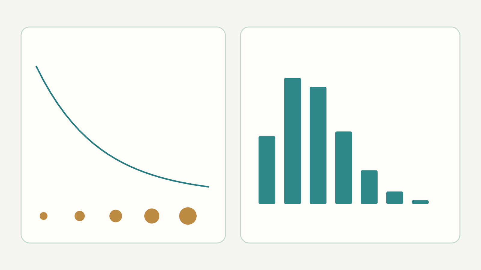
From questions to data, averages, expected goals and probabilities: build a Poisson model explaining every choice, symbol and operation.

1. Question before formula
We estimate each team’s goals and derive outcome probabilities. H denotes the home team, A the away team; G_H and G_A are their goals, non-negative integers. We cover 90 minutes plus stoppage time, excluding extra time and penalties. Defining the event prevents comparisons of different quantities.
The experimental poisson-v1 model uses results, not a neural network. It does not automatically include news, injuries, line-ups, motivation, opponent strength or odds. Its “expected goals” are modelled means, not shot-based xG.
2. Which data may enter
For the home team we use only home matches; for the away team only away matches. We use the same competition, completed matches and a 730-day window. GF means goals scored by the studied team; GS means goals conceded by that team. In an away-team row, GF is therefore not the score of the first-named team in the fixture.
cutoff = min(calculation time, kickoff time) − 4 hours
The cutoff is the latest admissible history time for the means. min chooses the earlier instant. The four hours are a precaution of this version, not a statistical law. A match timestamp alone does not prove its result was available: a real system must record when each piece of information arrived.
3. A dictionary before calculating
| Quantity | Meaning |
|---|---|
| GF / GS | Goals scored / conceded by the studied team |
| d, h, w | Age in days, half-life in days, match weight |
| W, F, C | Total weight, weighted goals scored, weighted goals conceded |
| μ_H, μ_A | Reference means: home, away |
| m, α | Added reference weight; fraction attributed to team |
| Attack / Defence | Relative factor for scored / conceded goals |
| λ_H, λ_A | Predicted goal means, not exact scores |
| P, q, Z, M | Probability; score product; grid sum; normalised cell |
Σ means “add all terms”. Subscript i identifies a match: w_i is its weight. exp(x) means e raised to x, where e is about 2.71828; ln is the natural logarithm, the inverse operation. A scientific calculator handles these functions.
4. Give recent matches more weight
A weight measures how much a match counts in the mean, not its winning probability. d is age in days relative to cutoff. h=180 days is the half-life: weight halves every 180 days. Times use UTC; divide the difference in seconds by 86,400.
w = exp(−ln(2) × d / 180) = 2^(−d/180)
d=0 → w=1; d=90 → w≈0.707107; d=180 → w=0.5; d=360 → w=0.25
A 360-day-old match counts one quarter as much as a new one. W, total weight, may be far below the match count: it is not a number of independent observations. The 180-day choice must be tested, not accepted for appealing results.
5. Build a weighted mean
Multiply each goal count by its match weight. Add the products, then divide by total weight, not the match count. F collects weighted goals scored; C weighted goals conceded.
W=Σw_i; F=Σ(w_i × GF_i); C=Σ(w_i × GS_i)
mean_GF=F/W; mean_GS=C/W
A made-up teaching example: 1 goal with weight 1; 3 goals with weight 0.5. The simple mean is (1+3)/2=2. The weighted mean changes because the second match counts less.
W=1+0.5=1.5
F=1×1+0.5×3=2.5
F/W=2.5/1.5≈1.666667
6. The competition reference
A reference is needed to judge a mean. Calculate separate competition means for home goals μ_H and away goals μ_A using the same temporal rules and weights. S_H and S_A are weighted goal sums; W_L is competition total weight.
μ_H=S_H/W_L; μ_A=S_A/W_L
μ_H≈2.000320947500; μ_A≈1.346459586694
The 537 competition matches are available as aggregates, not all underlying rows. We can repeat divisions, but cannot audit every match or recalculate the reference with a different half-life from aggregates alone.
7. Do not trust a tiny sample too much
Regularisation pulls an uncertain mean towards the reference. Add reference weight m=8. F is the weighted goal sum, W the team weight and μ the relevant reference. m is not a mathematical constant: compare this choice on data later than the training data.
adjusted_mean=(F+mμ)/(W+m)
=F/(W+m)+mμ/(W+m)
=[W/(W+m)]×(F/W)+[m/(W+m)]×μ
α=W/(W+m); 1−α=m/(W+m)
adjusted_mean=α(F/W)+(1−α)μ
The second form explains the first: α is the team contribution, 1−α the reference contribution. If W=2 and m=8, α=2/10=0.2 and α×100%=20%, versus 80% reference. Add mμ above and m below because we add weight with mean μ, not eight goals.
8. Attack and defence: four divisions
| Quantity | Formula | μ |
|---|---|---|
| Home attack | Attack_H=((F_H+8μ_H)/(W_H+8))/μ_H | μ_H |
| Home conceded | Defence_H=((C_H+8μ_A)/(W_H+8))/μ_A | μ_A |
| Away attack | Attack_A=((F_A+8μ_A)/(W_A+8))/μ_A | μ_A |
| Away conceded | Defence_A=((C_A+8μ_H)/(W_A+8))/μ_H | μ_H |
Dividing by reference gives a unit-free factor: 1 means equal, 1.20 means 20% more. High attack means more goals scored; high defence means more conceded, hence vulnerability, not strength. A home team concedes away-team goals, and vice versa: mind the denominators.
9. Combine the opponents
λ, Greek lambda, is the predicted goal mean. Multiply reference by team attack and opponent vulnerability. 1.8 does not mean scoring eight tenths of a goal: it is a mean over possible integer outcomes.
λ_H=μ_H × Attack_H × Defence_A
λ_A=μ_A × Attack_A × Defence_H
λ_used=max(0.15, min(5, λ))
The last line clips the mean to 0.15–5: min chooses smaller and max larger. It is a safeguard, not proof of accuracy. It changes neither example.
10. From mean to goal counts
Poisson assigns probabilities to counts 0, 1, 2, 3… given a positive mean λ. k is the requested count; k! is factorial: 3!=3×2×1=6 and by definition 0!=1. P(G=k) means “probability of k goals”. Choosing this distribution is an assumption to test.
P(G=k)=exp(−λ) × λ^k/k!
P(G=0)=exp(−λ)
P(G=k)=P(G=k−1) × λ/k
The last formula avoids repeated powers and factorials: start at zero, then move to the next count. Teaching example with λ=2:
P(0)=exp(−2)≈0.135335
P(1)=P(0)×2/1≈0.270671
P(2)=P(1)×2/2≈0.270671
P(2) × 100% ≈ 27.0671%
11. The score matrix
Assume independent goal counts: knowing one does not change the other distribution. This can be imperfect in football. Under this assumption multiply count probabilities. i denotes home goals, j away goals: (i,j) is an exact score.
q(i,j)=P(G_H=i) × P(G_A=j)
Z=Σ q(i,j), 0≤i≤30, 0≤j≤30
M(i,j)=q(i,j)/Z
Use 0–30 goals per team: 31×31=961 cells. Z is their total. Dividing each by Z restores a total of 1: we truncate and renormalise an infinite distribution, not declare more than 30 goals impossible. At these means the excluded mass is numerically negligible.
12. Add the right cells
| Event | Meaning | Formula |
|---|---|---|
| 1 | Home wins: i>j | P1=Σ M(i,j), i>j |
| X | Draw: i=j | PX=Σ M(i,i) |
| 2 | Away wins: i<j | P2=Σ M(i,j), i<j |
| 1X / X2 / 12 | Double chances | P1+PX / PX+P2 / P1+P2 |
| Over 2.5 | At least 3 total goals | Σ M(i,j), i+j≥3 |
| GG | Both teams score | Σ M(i,j), i≥1, j≥1 |
1, X and 2 are exclusive and exhaustive: total 1, or 100%. Double chances 1X, X2 and 12 overlap: every single outcome appears twice. Their total is 2, or 200%: not an error. Always show percentage conversion p×100%.
We defined the calculations, not their reliability. Stage 2 executes them with all the numbers; stage 3 explains how to test them.
Before continuing: try it
1. What does a match with weight 0.5 and 4 goals add to F and W?
Show the explanation
It adds 0.5×4=2 to F and 0.5 to W. The final mean is F/W, not F divided by match count.
2. Why does home defence use μ_A?
Show the explanation
Because goals conceded by the home team are scored by away teams. A defence factor above 1 means more conceded, not better defence.
3. With W=2 and m=8, how much does the reference count?
Show the explanation
α=2/(2+8)=0.2; team weight 0.2×100%=20%. Reference weight (1−0.2)×100%=80%. m=8 adds weight, not eight goals.
4. Why does 1X+X2+12 give 200%?
Show the explanation
Each simple outcome occurs twice: (P1+PX)+(PX+P2)+(P1+P2)=2(P1+PX+P2)=2. Thus 2×100%=200%. Double chances are not disjoint.