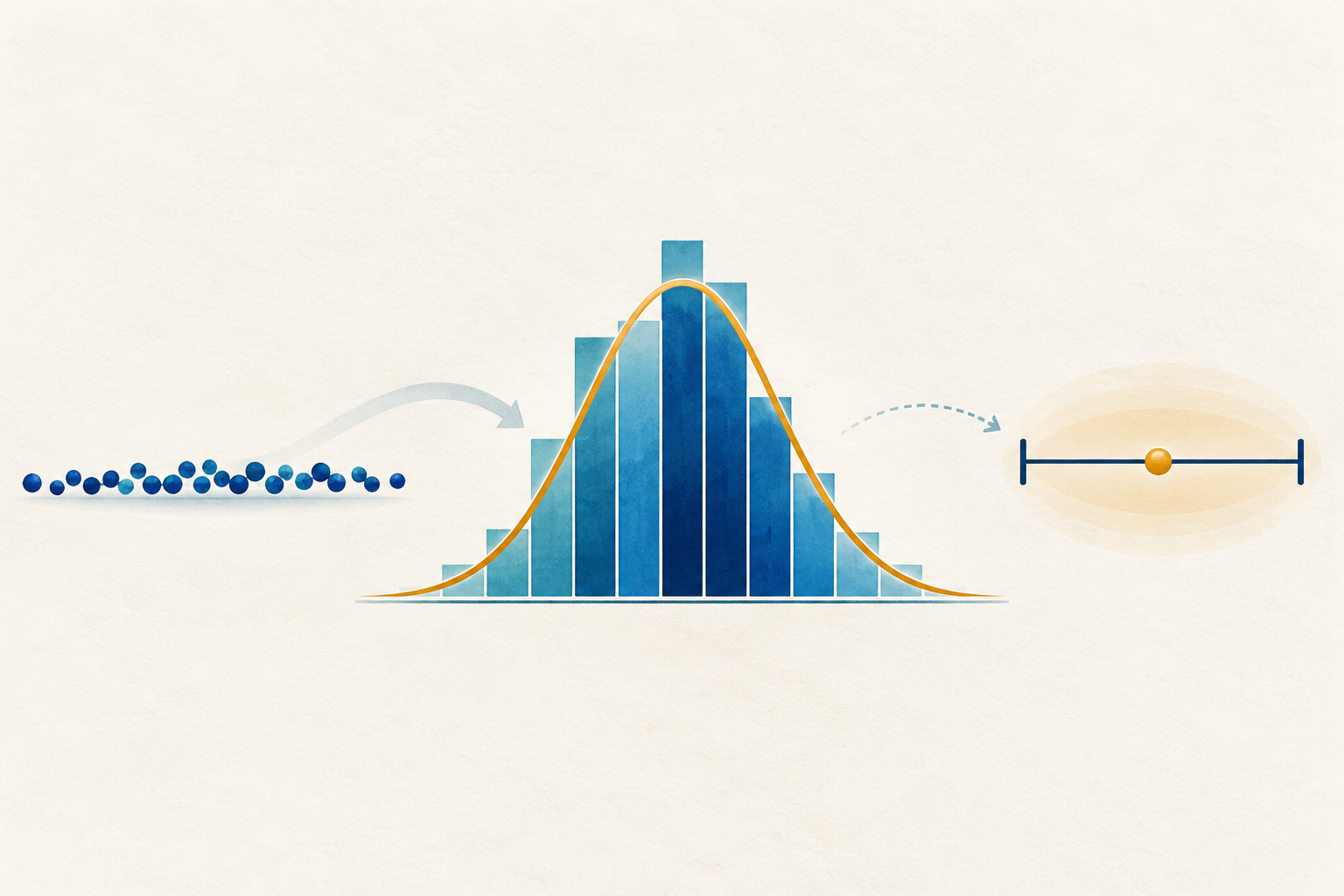
We collect a set of measurements. We draw a histogram, and a curve seems to follow it closely. Have we discovered the law governing the phenomenon? Not yet. We have built one possible model, to be compared with others and interpreted in light of how the data were collected. The distribution laboratory lets us follow this path using our own numbers.
From sample to population
The population is the group about which we want to draw a conclusion; the sample contains the n observations actually available. The sample mean x̄ estimates the unknown population mean μ. The sample standard deviation s describes how widely values spread around x̄. Another sample might yield another mean: that is why a point estimate does not convey all the uncertainty.
Before calculating, ask whether observations are independent, whether the sample is representative and whether every value has the same meaning. A flawless calculation cannot repair a badly selected sample.
What does a histogram tell us?
A histogram groups measurements into intervals. In the laboratory, bar heights represent densities, so the total bar area is 1 and continuous curves can be overlaid. The shape also depends on the choice of bins: an apparent bell shape does not, by itself, prove Normality.
For continuous measurements the laboratory tries Normal, Uniform and Exponential models; when every value is strictly positive it also includes Lognormal and Weibull. Integer counts have a separate tab: Poisson and, when the number of trials per observation is known, Binomial. A continuous density curve and the probabilities of individual counts are not the same thing.
The distributions at a glance
A distribution models the probabilities of possible outcomes. Start with the type of data, not the name of a curve: a measurement can vary continuously, while a count takes only whole-number values.
- Normal: a symmetric bell-shaped model described by mean μ and standard deviation σ.
- Uniform: within an interval [a, b], subintervals of equal width have equal probability.
- Exponential: describes nonnegative waiting times when the event rate remains constant; its parameter is λ.
- Lognormal: describes positive values whose logarithms follow a Normal distribution; it often has a long right tail.
- Weibull: models positive lifetimes; shape and scale allow different profiles.
- Poisson: counts events in a fixed interval using a mean event count λ.
- Binomial: counts successes in m independent trials, each with success probability p.
Comparing models without declaring an absolute winner
Each model has parameters estimated from the data. The laboratory compares the observed cumulative distribution with that of the model using a distance D: among the candidates shown, a smaller D indicates a better descriptive match. It does not prove that the model is the true distribution, and it is not a p-value. In particular, the parameters were estimated from the same sample, so the critical values of the standard Kolmogorov–Smirnov test cannot simply be applied.
Read this comparison alongside the histogram, the nature of the phenomenon and the sample size. If plausible models are missing, even the first-ranked candidate may be inadequate.
The chi-square test: observed versus expected
If outcomes are divided into categories and the null hypothesis H₀ probabilities are fixed before seeing the data, we can compare observed frequencies O with expected frequencies E = N × p. The statistic is χ² = Σ (O − E)² / E: large discrepancies relative to expected counts give a larger value. The p-value says how unusual a discrepancy at least this large would be if H₀ were correct; it is not the probability that H₀ is true.
In the chi-square test laboratory you can follow the calculation category by category and try a die, a Poisson model with known λ and a Binomial model with known parameters. Observations must be independent and every expected count at least 5. If parameters are estimated from the same data, as in the fitted models above, degrees of freedom require different treatment: do not reuse this laboratory’s simple p-value for those models. NIST reference.
An interval for the mean, not for individual observations
The mean x̄ is one number; a confidence interval adds a margin expressing uncertainty in the estimate of μ. If the population standard deviation σ is known, the two-sided interval uses a critical z value and standard error σ/√n. More commonly σ is unknown: we use s and a critical value from Student’s t distribution with n−1 degrees of freedom:
CI for μ = x̄ ± t1−α/2,n−1 · s/√n.
The laboratory offers 90%, 95% and 99% confidence levels. With the same data, more confidence means a wider interval; as n grows, standard error tends to decrease. For small samples, the t method calls for particular care with the assumption of an approximately Normal population.
A step-by-step calculation
Suppose we have n = 16 weights with x̄ = 75 kg and s = 12 kg, without knowing σ. Standard error is 12/√16 = 3 kg. At 95% confidence, with 15 degrees of freedom, the critical value is about 2.1314. The margin is 2.1314 × 3 ≈ 6.39 kg and the interval is [68.61, 81.39] kg.
If σ = 12 kg were genuinely known independently of this sample, we would instead use z ≈ 1.9600, giving [69.12, 80.88] kg. And with n = 100, keeping x̄ = 75 kg and s = 12 kg, the 95% t interval would be about [72.62, 77.38] kg. This is not magic: under the method’s assumptions, more data reduce standard error.
What does “95%” really mean?
The population mean μ does not change after we inspect the sample. The 95% describes the procedure: if we repeatedly drew samples under the same conditions, approximately 95 out of 100 intervals built this way would contain μ. It does not mean that 95% of people have values inside this interval, nor does it assign a 95% probability to an already fixed μ.
If the data are strongly skewed, contain outliers or come from a biased sample, the classical interval may mislead. The laboratory flags some cautions, but it cannot determine by itself how the sampling was designed.
Test the ideas yourself
In the interactive laboratory you can paste 5 to 2,000 measurements, inspect their histogram and models, and calculate a confidence interval for the mean; alternatively, enter n, x̄ and s or σ directly when you have only summary statistics. A separate tab analyzes counts, while the “Test me” mode conceals the generating distribution. Seven worked examples show how intervals change. Data entered in the laboratory stay in your browser.
Open the distribution and confidence interval laboratory
Further reading: NIST, confidence limits for the mean and NIST, limitations of the Kolmogorov–Smirnov comparison.