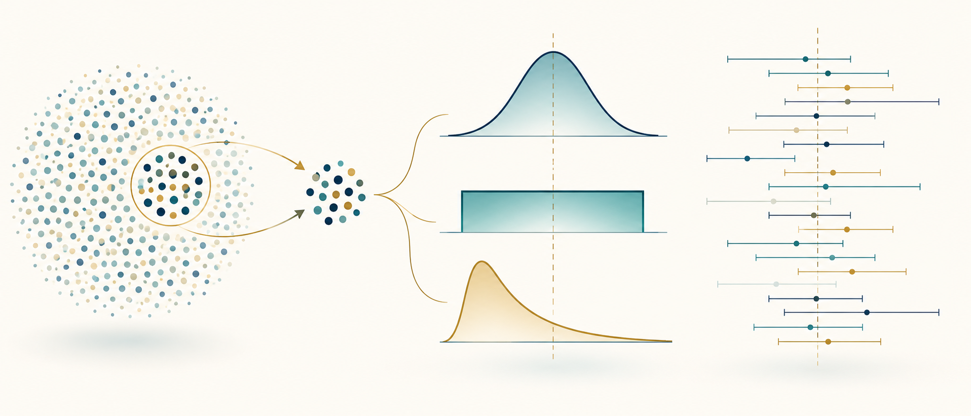
A probability curve does not arise from a histogram: it is a model we use to describe a phenomenon and make predictions. The next step is to understand what we can learn by observing only a sample. We will follow one thread: population → random variable → distribution → sample → sample statistic → sampling distribution of the statistic → confidence interval. By the end, every formula will have a meaning and every simulation a precise question.
1. Experiment, random variable and distribution
A random experiment has an uncertain outcome before observation, even under defined conditions. A random variable X assigns a number to each possible outcome: a success count, a waiting time, a measurement. If its possible values are isolated, X is discrete; if it can take values across an interval, it is continuous. A distribution assigns probabilities to possible values. For a discrete variable we use P(X = x); for a continuous one we use a density f(x), whose area over an interval is a probability. In general P(X = x) = 0 for a single continuous value.
The cumulative distribution function F(x) = P(X ≤ x) accumulates probability up to x. The theoretical mean E(X) locates the distribution; the variance Var(X) measures squared dispersion; the standard deviation is its square root. These are properties of the model, not values that change with each sample. A useful laboratory keeps formula, parameters, graph, meaning and simulated data visible together.
2. The eight basic distributions
Bernoulli. One trial has two outcomes, coded 1 (success) and 0 (failure), with success probability p, 0 ≤ p ≤ 1. P(X=1)=p; P(X=0)=1−p; E(X)=p; Var(X)=p(1−p). Example: a correct or incorrect answer. Simulate many trials and compare the success fraction with p: they need not be identical in every sequence.
Binomial. Counts successes in n independent Bernoulli trials with the same p. For k from 0 to n, P(X=k)=C(n,k)p^k(1−p)^(n−k); E(X)=np; Var(X)=np(1−p). Example: successes in 20 tosses or answers. Change n and p to see how the shape changes and how simulated frequencies approach theoretical probabilities.
Poisson. Counts events in a fixed interval when the model assumes independent events at a constant average rate λ > 0. For k = 0,1,2,…, P(X=k)=e^(−λ)λ^k/k!; E(X)=λ; Var(X)=λ. Example: arrivals during a time window. Change λ and observe centre and spread; do not confuse the event count with the time between arrivals.
Continuous uniform. On [a,b], where a < b, intervals of equal length have equal probability: f(x)=1/(b−a) inside [a,b] and zero outside; E(X)=(a+b)/2; Var(X)=(b−a)^2/12. Simulate a sample and compare its imperfectly flat histogram with the perfectly flat theoretical density.
Normal or Gaussian. Continuous and symmetric around mean μ, described by μ and σ > 0: f(x)=[1/(σ√(2π))] exp(−(x−μ)^2/(2σ²)); E(X)=μ; Var(X)=σ². Move μ to shift the bell and vary σ to widen it. Its importance for sample means does not imply that every real phenomenon is Normal.
Exponential. Continuous and nonnegative; in a constant-rate event model it describes waiting time with λ > 0: f(x)=λe^(−λx) for x ≥ 0 and zero otherwise; E(X)=1/λ; Var(X)=1/λ². Simulate waiting times and observe the right tail. Poisson counts events; Exponential measures a wait in the corresponding model.
Student t. Continuous and symmetric, depending on degrees of freedom ν. For independent Normal observations with unknown σ, T=(x̄−μ)/(s/√n) follows a t distribution with ν=n−1. Its mean is zero if ν > 1 and its variance is ν/(ν−2) if ν > 2; at small ν its tails are heavier than those of the Normal. Overlay t and the standard Normal as ν increases: the difference shrinks.
Chi-square. If Z₁,…,Zν are independent standard Normals, χ²=Z₁²+⋯+Zν² has ν degrees of freedom; E(χ²)=ν; Var(χ²)=2ν. It is positive and skewed, especially for small ν. It is useful in studying variance and in some tests: do not identify the distribution with every application of a chi-square test. The dedicated laboratory compares observed and expected frequencies.
3. From model to observed data
The theoretical distribution describes a model; a sample of size n is one possible realisation: X₁,…,Xₙ. We compute x̄=(X₁+⋯+Xₙ)/n and s²=Σ(Xᵢ−x̄)²/(n−1). The denominator n−1 makes s² an unbiased estimator of the variance under independent identically distributed sampling. A new sample from the same model changes x̄, s² and the histogram: this variability is not a software error.
Try an experiment: choose a distribution and parameters, generate a sample, record x̄ and s, then request a new sample without changing the model. Repeat. The population parameter stays fixed; the calculated statistics change. One set of 100 observations does not mean 100 populations.
4. The sampling distribution of the mean
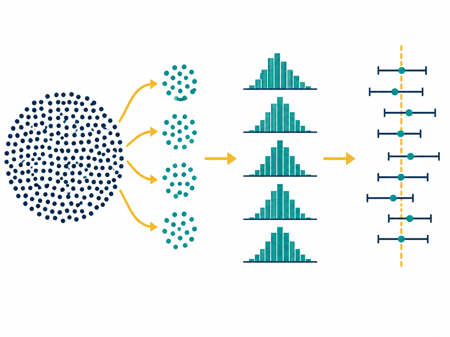
Now repeatedly draw whole samples of the same size n, retaining only one mean per sample. The resulting histogram does not describe individual observations: it describes the sampling distribution of x̄. For independent identically distributed samples with mean μ and finite variance σ², E(x̄)=μ and SD(x̄)=σ/√n. This last quantity is the mean’s standard error. Quadrupling n halves the standard error; it does not eliminate it.
The central limit theorem says that, under suitable conditions, the distribution of the standardised mean approaches a Normal as n increases. If the population is Normal, the mean is Normal for every n; with a uniform or exponential population we can watch the approach instead. Compare n = 2, 5, 30 and 100 using many samples, placing the histogram of individual values next to that of the means. Strong skewness or dependence may make the approximation slow or unsuitable.
5. Why a confidence interval?
A sample mean estimates μ but says nothing by itself about its precision. A confidence interval builds a band around x̄ that varies from sample to sample. Its level, for example 95%, is the long-run coverage of the procedure in ideal repetitions of the same experiment under the model assumptions. Once an interval has been observed, μ is a fixed value: we do not say it has a 95% probability of lying in that interval. Nor do we say that 95% of individual observations lie there.
6. Mean with known σ: the z interval
When the population standard deviation σ is genuinely known and the population is Normal, or n is large enough for the approximation, the two-sided interval is x̄ ± z_(1−α/2)·σ/√n at level 1−α. Common critical values are 1.645 at 90%, 1.960 at 95% and 2.576 at 99%. The margin of error grows with the required level and with σ, and shrinks with √n. A sample-based s must not be presented as a σ known in advance.
Example. For n=100, x̄=50, σ=10, at 95% the standard error is 1 and the margin 1.960: the interval is [48.04, 51.96]. At 99% the margin becomes 2.576 and the interval widens. Coverage is gained, not precision.
7. Mean with unknown σ: the t interval
In practice σ is often unknown. Use the sample standard deviation s and a Student t quantile: x̄ ± t_(1−α/2,n−1)·s/√n. There are n−1 degrees of freedom. For a small sample, exact justification requires a Normal population; larger samples still require independence and attention to tails, outliers and sampling design. The heavier t tails generally yield a wider interval than z for the same data.
Example. For n=16, x̄=75, s=12, the standard error is 12/√16=3. At 95%, with 15 degrees of freedom, t≈2.131; the margin is about 6.39 and the interval [68.61, 81.39]. Repeat a z/t comparison at n = 5, 10, 30 and 100: the differences shrink as n grows.
8. See coverage rather than merely read about it
Fix a population whose mean μ is known to the simulator, choose n and a level (90%, 95% or 99%), then draw 10, 100, 1,000 or 10,000 independent samples. Build an interval for each sample. In a horizontal plot draw μ as a vertical line; use one colour for intervals that cross it and another for those that miss it. Observed coverage is intervals containing μ / all intervals. It need not equal 95% in a run of ten; across many repetitions it approaches the nominal level if assumptions hold.
Three guided experiments: decrease n and watch intervals lengthen; raise the confidence level and compare width and coverage; switch from z to t when σ is unknown and notice the cost of extra uncertainty. A t coverage simulation must recalculate s for every sample rather than reuse a single standard deviation.
9. Organising the laboratory
Six interactive modules make the conceptual transitions natural. Explore a distribution: choose among eight distributions, change parameters and read formula, shape and mean. Generate a sample: choose n and inspect its histogram, x̄, s² and s. Repeat sampling: collect many means and compare them with individual data. Build an interval: set 90%, 95% or 99%, consciously select known or unknown σ and inspect each term. Check coverage: repeat sampling and colour intervals according to whether they cover μ. Guided experiments: answer questions such as ‘What changes if I double n?’ and ‘Why is 99% wider than 95%?’, then check with graphs.
Charts readable on a phone, sliders displaying their values, ‘New sample’, ‘Repeat 100’, ‘Repeat 1,000’ and ‘Reset’ buttons, short explanations by each result and distinct colours for theoretical parameters, samples and intervals are more useful than a spectacular graph. An optional random seed makes an experiment reproducible. The existing laboratory supports data analysis, model comparison and interval calculation; repeated sampling and coverage modules described here are proposed teaching extensions, not features presumed to exist already.
10. Teaching specification for later development
The basic simulations can run entirely in the browser without a database. The interface should let users select distribution, parameters and sample size; generate one sample and repeat 100 or 1,000 times; clearly separate theoretical density/probabilities, observed histogram and histogram of means; show standard error and z/t intervals step by step; and compare observed and expected coverage without presenting one run as a law. All eight distributions require parameter-domain checks and numerical tests; intervals require checks of quantiles, degrees of freedom and edge cases. A stable charting library may draw responsive plots, but statistical formulas must be implemented and verified explicitly.
An ‘Explain it’ panel should connect each control to a question: ‘What stays fixed in the population?’, ‘What changes between samples?’, ‘Which distribution does this histogram describe?’, ‘What does 95% mean?’. The interface should teach interpretation, not merely output answers.
11. Possible extensions
After the basic level, one might add intervals for a proportion, chi-square intervals for variance, comparisons of two means or proportions, bootstrap, hypothesis tests, goodness-of-fit tests, CSV import and Q-Q plots. Each extension needs its own assumptions; it is not simply another button applied indiscriminately to the same data. The natural link with the existing laboratory is to move thoughtfully from data exploration to inference.
Conclusion
Theory tells us what to expect; simulation shows what actually varies; an interval quantifies the uncertainty of an estimate. Before clicking, always ask what the population is, which variable is being measured, how the sample was drawn and which statistic is being observed. That chain, not an isolated formula, makes applied probability understandable.