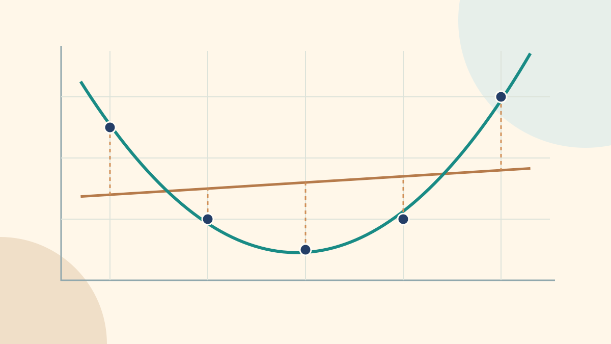
Two points do not tell us which path to follow between them: a line and a curve may share endpoints but give different estimates in between. With noisy measurements, insisting on an exact fit may be even less appropriate.

We separate three questions: constructing a function through specified points, fitting a model to observations, and using it outside the observed range. Starting with elementary examples, we reach quadratic regression y=ax²+bx+c using least squares. All datasets are teaching examples, not real-world forecasts.
1. Interpolation, regression and extrapolation are not synonyms
Interpolation imposes an exact fit at chosen nodes; the function family determines whether the result is unique. Two distinct x values specify one line; three specify one polynomial of degree at most two. Without choosing a family, infinitely many curves are possible.
Regression estimates parameters from all observations, generally allowing residuals. Interpolating or extrapolating a prediction describes where the requested x lies: a regression line can predict inside or outside the observed range. Being inside the range does not automatically make a function an interpolant.
| Idea | What it imposes | What it does not guarantee |
|---|---|---|
| Interpolation | Exact fit at chosen nodes within a stated family. | A valid physical model between nodes. |
| Regression | Overall fit under an error criterion. | Passing through every point or causal validity. |
| Extrapolation | Using a model outside its node/data interval. | Continuation of the observed behaviour. |
2. Linear interpolation in four steps
Take (2,100) and (6,200) and estimate at x=3. Assuming constant absolute increments means choosing a line.
1. Vertical difference: 200−100=100. 2. Horizontal interval: 6−2=4. 3. Slope: m=100/4=25. 4. Move 3−2=1 unit from the first endpoint: y=100+25×1=125. The line is y=25x+50. The endpoint x values must differ.
y = y₁ + [(y₂−y₁)/(x₂−x₁)] × (x−x₁)
y = 100 + [(200−100)/(6−2)] × (3−2) = 1253. Exponential interpolation: logarithms first
Constant ratios over equal x increments suggest y=A exp(kx), A>0. Taking logarithms gives ln(y)=ln(A)+kx, a line in the (x,ln y) plane. Applying exp returns to the original quantity.
For the same endpoints, t=(3−2)/(6−2)=1/4 and y=100×2^(1/4)≈118.92, not 125. At x=4 the line gives 150, while the exponential gives √(100×200)≈141.42: arithmetic versus geometric mean. Logarithms require positive y.
k is the logarithmic change per x unit; the multiplicative factor is exp(k). For k>0 the doubling time is ln(2)/k; for k<0 the half-life is ln(2)/|k|. These properties are useful only when the model is appropriate.
ln(y) = ln(A) + kx
k = [ln(y₂)−ln(y₁)]/(x₂−x₁)
t = (x−x₁)/(x₂−x₁)
y = y₁ × (y₂/y₁)^t
y(3) = 100 × 2^(1/4) ≈ 118.920712
4. Power laws: transform both axes
For y=A x^p, with A>0 and x>0, transform x too: ln(y)=ln(A)+p ln(x). The slope in the (ln x,ln y) plane is p, not the exponential model’s k.
The endpoints (2,4),(8,64) give p=ln(64/4)/ln(8/2)=2 and A=1. At x=4 the power law gives 16; the endpoint line gives 24. Doubling x multiplies y by 2^p: four when p=2, √2 when p=1/2.
p is also elasticity: for a small 1% rise in x, y changes by approximately p%. For a fractional change h the exact factor is (1+h)^p, not generally 1+ph.
ln(y) = ln(A) + p ln(x)
p = ln(y₂/y₁)/ln(x₂/x₁)
A = y₁/x₁^p
y(x) = y₁ × (x/x₁)^p
y(4) = 4 × (4/2)² = 16
5. Ordinary, semilog and log-log scales
Equal distances on an ordinary axis mean equal differences; on a logarithmic axis they mean equal ratios. For example 1,10,100,1000 are equally spaced on a base-10 log axis. Zero and negative values cannot be shown there.
An exponential appears straight with ordinary x and logarithmic y. Using log₁₀(y), its slope is k/ln(10); using ln(y), it is k. A power law appears straight on log-log axes, with slope p when both axes use the same base.
Changing the graph scale does not refit coefficients. Choosing to minimize log-space errors is a different operation: it changes the fitting criterion, not merely the picture.
| Model | Equation | Straight-line transformation |
|---|---|---|
| Line | y=mx+q | None |
| Exponential | y=A exp(kx) | Y=ln(y), X=x |
| Power | y=A x^p | Y=ln(y), X=ln(x) |
| Quadratic | y=ax²+bx+c | Linear in parameters, not straight in x |
6. Clues for choosing a model, not proofs
With equal x steps, roughly constant y differences suggest a line and roughly constant ratios suggest an exponential. Straightness on log-log axes suggests a power law. These are clues to investigate, not proofs.
Compound growth, some decay processes and certain growth phases can motivate exponentials; geometry and scaling relations can motivate powers. A parabola may describe local curvature, but cannot automatically be extended indefinitely. Context and new data must challenge the model.
7. Regression and least squares
For observation i, let ŷᵢ=f(xᵢ) and rᵢ=yᵢ−ŷᵢ, its vertical residual. Least squares chooses parameters minimizing S=Σrᵢ². Squaring prevents positive and negative residuals cancelling and gives larger residuals greater influence.
For y=mx+q the coefficients follow from means and sums of deviations. The line is not required to pass through every observation. This criterion minimizes vertical y deviations, not perpendicular distances to the line.
For exponential and power models, this laboratory fits a line to logarithms, minimizing Σ[ln(yᵢ)−ln(ŷᵢ)]². This is generally not the same as minimizing Σ(yᵢ−ŷᵢ)². It does not perform nonlinear least squares on original y or a retransformation-bias correction.
S = Σᵢ[yᵢ−f(xᵢ)]² → min
m = Σ(xᵢ−x̄)(yᵢ−ȳ) / Σ(xᵢ−x̄)²
q = ȳ − mx̄
8. Quadratic regression: finding a, b and c
Quadratic regression seeks y=ax²+bx+c minimizing S(a,b,c)=Σ[yᵢ−(axᵢ²+bxᵢ+c)]². The curve is not straight in x, but the fitting problem is linear in a,b,c: these parameters appear to the first power and are not multiplied together.
Setting three partial derivatives to zero yields three normal equations. Their sums use all observations. A unique fit requires at least three distinct x values; three measurements at one x are insufficient.
Example: x=−2,−1,0,1,2 and y=5,2,1,2,6. The sums are n=5, Σx=0, Σx²=10, Σx³=0, Σx⁴=34, Σy=16, Σxy=2, Σx²y=48. Thus 34a+10c=48; 10b=2; 10a+5c=16. Solving gives a=8/7, b=1/5, c=32/35.
The residual sum of squares is 4/35≈0.114286; the regression line on these same points is y=0.2x+3.2 with S=18.4. The parabola fits this sample better, but that comparison alone does not establish better prediction on new data.
Normal equations explain the calculation. Numerically, the laboratory centers and scales x and uses QR factorization rather than directly solving the more conditioning-sensitive sum system.
y = ax² + bx + c
S(a,b,c) = Σᵢ[yᵢ−(axᵢ²+bxᵢ+c)]² → min
∂S/∂a = −2Σxᵢ²[yᵢ−(axᵢ²+bxᵢ+c)] = 0
∂S/∂b = −2Σxᵢ[yᵢ−(axᵢ²+bxᵢ+c)] = 0
∂S/∂c = −2Σ[yᵢ−(axᵢ²+bxᵢ+c)] = 0
aΣx⁴ + bΣx³ + cΣx² = Σx²y
aΣx³ + bΣx² + cΣx = Σxy
aΣx² + bΣx + nc = Σy34a + 10c = 48
10b = 2
10a + 5c = 16
a = 8/7; b = 1/5; c = 32/35
y = (8/7)x² + (1/5)x + 32/35| x | y | ŷ | r=y−ŷ | r² |
|---|---|---|---|---|
| -2 | 5 | 5.085714 | -0.085714 | 0.007347 |
| -1 | 2 | 1.857143 | 0.142857 | 0.020408 |
| 0 | 1 | 0.914286 | 0.085714 | 0.007347 |
| 1 | 2 | 2.257143 | -0.257143 | 0.066122 |
| 2 | 6 | 5.885714 | 0.114286 | 0.013061 |
9. Three exact points or many observations?
For three distinct x values, a quadratic interpolant passes through all three points. Quadratic regression on those same three points coincides with it up to rounding. Degree at most two includes a line when a=0.
Five observations need not lie on one parabola: least squares finds the best fit under the chosen criterion. Laboratory quadratic interpolation uses only three chosen nodes; other points remain comparisons. Linear, exponential and power interpolants use two nodes.
Piecewise linear interpolation joins all ordered nodes with segments; splines join polynomial pieces. Neither is the single line or parabola compared here. High-degree polynomial interpolation can oscillate: greater complexity does not automatically bring reliability.
10. Residuals, fit quality and limitations
The lab shows residuals, SSE=Σrᵢ², RMSE=√(SSE/n) and R²=1−SSE/Σ(yᵢ−ȳ)², computed in original units over all entered points. This RMSE is not a residual standard-deviation estimate adjusted for degrees of freedom.
When all y values coincide, R² has a zero denominator and is reported as undefined. For log-fitted models, original-scale R² can be negative. A high R² establishes neither causation nor validity outside the data.
A single unusual observation may shift least-squares coefficients substantially. Curved patterns or other structure in residuals suggest a poor model. Check unused data and uncertainty: this lab does not compute confidence or prediction intervals.
11. One laboratory, six meaningful experiments
Load the endpoint example and switch line to exponential: compare 125 and 118.92 at x=3. Then load the power example and inspect its value at x=4 on all three graph scales.
Load the noisy parabola, compare linear and quadratic regression, and inspect a,b,c and the numeric normal equations. Switch to three-node interpolation: those nodes are exact constraints, not necessarily the two remaining observations.
Use noisy growth to examine a straight semilog graph and distinguish original SSE from the log-space objective. Finally try extrapolation and the unusual-point example; edit a value and inspect coefficients and residuals. There are six editable experiments.
Open the lab: points, curves, residuals and steps
12. Try it: five problems with hidden solutions
Try before revealing answers. First ask which points are constraints, which family is being chosen and where the requested x lies.
1. Between (1,10),(5,30), what does the line give at x=2?
Show solution and explanation
m=(30−10)/(5−1)=5. y=10+5×(2−1)=15.
2. Between (0,50),(4,800), what does the exponential give at x=2?
Show solution and explanation
t=1/2. y=50×(800/50)^(1/2)=200: the geometric mean, not the arithmetic mean 425.
3. Between (1,3),(4,48), which power law and value at x=2?
Show solution and explanation
p=ln(48/3)/ln(4/1)=2; A=3. Thus y=3x² and the value is 12.
4. Do three distinct x values always give a unique quadratic interpolant?
Show solution and explanation
They give one polynomial of degree at most two, possibly a line. Quadratic regression on the same three points gives that polynomial, apart from rounding.
5. Does changing ordinary axes to logarithmic axes refit a regression?
Show solution and explanation
No: it changes only the display. Fitting on logarithms instead changes the objective. These operations must not be confused.