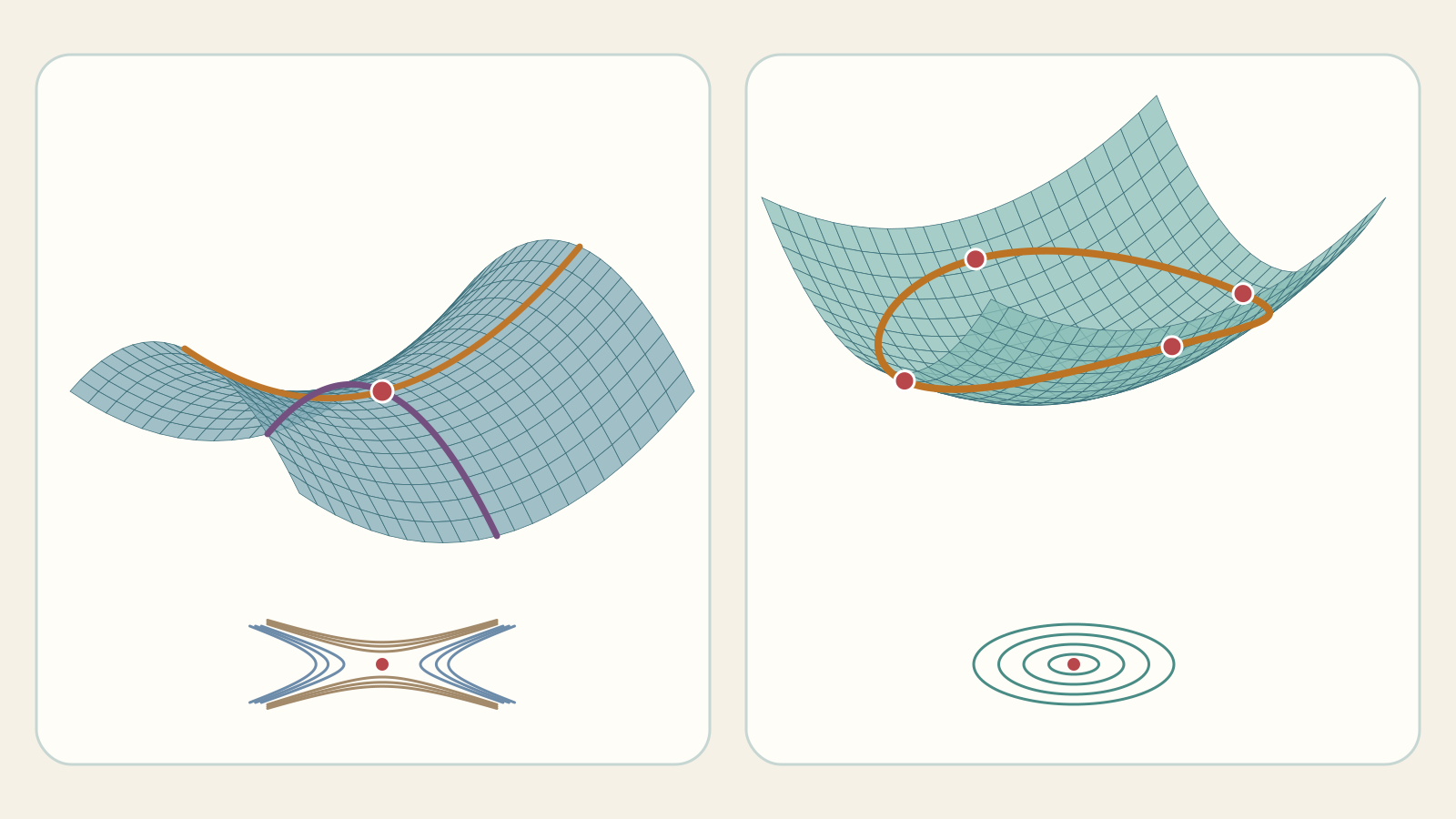
What is the largest or smallest value a function can attain? With two variables, setting one derivative to zero is not enough: we need to know which movements are allowed and compare every candidate. Stage 22 connects the gradient to extrema, first unconstrained and then constrained.
Maxima and minima: laboratory · Learning-path index
1. What are we seeking, and on which set?
An optimization problem has an objective f and a feasible set E. The point P must belong to E. A global minimum means f(P) ≤ f(Q) for every Q in E; a global maximum reverses the inequality. A local extremum compares only sufficiently nearby feasible points.
min: P∈E, ∀Q∈E: f(P)≤f(Q)
max: P∈E, ∀Q∈E: f(P)≥f(Q)
An extremum is strict if equality is excluded at the other points being compared. An extremal point differs from an extremal value: for f=x²+y² the minimizing point is (0,0), the minimum value is 0. The same value may occur at multiple points. In constrained problems proximity is always within E.
2. Existence: Weierstrass and its limits
If E is nonempty, closed and bounded in ℝ² and f is continuous on E, Weierstrass guarantees both global extrema. It establishes existence, not their location or uniqueness. A closed disk includes its boundary; an open disk does not.
f=x²+y², E={x²+y²<1}: min f=0; sup f=1, 1∉f(E).
On the open disk 1 is a supremum but not a maximum: it is never attained. On ℝ² the same function has minimum 0 and no maximum. Failure to meet the hypotheses does not prove absence of extrema; this theorem simply gives no guarantee.
3. Free extrema: why the gradient must vanish
Suppose f is differentiable and P is interior to its domain. At a local extremum, restricting f to any line through P leaves a single-variable extremum. In particular the derivatives along both coordinate axes vanish. This is necessary, not sufficient.
fₓ(x,y)=0
fᵧ(x,y)=0
∇f(P)=(0,0)
Solutions are stationary points. Do not discard nondifferentiable points: f=√(x²+y²) has a minimum at the origin, where its gradient does not exist. Boundaries and nonsmooth points need separate study. All lab objectives are polynomials; a constraint can nevertheless be singular.
4. Hessian: the second-order test
If f is C² near a stationary point P, its second derivatives form the symmetric Hessian. Its determinant D helps decide whether the quadratic part of Taylor changes sign. This test concerns free interior points, not automatically constrained extrema.
H(P)=[ fₓₓ  fₓᵧ ; fₓᵧ  fᵧᵧ ]
D=fₓₓ fᵧᵧ−(fₓᵧ)²
D>0, fₓₓ>0 → strict local minimum
D>0, fₓₓ<0 → strict local maximum
D<0 → saddle
D=0 → inconclusive test
Why? At a stationary point f(P+h)−f(P)=½ hᵀH(P)h+o(‖h‖²). A positive definite quadratic form dominates the remainder and values increase in every nearby direction; a negative one decreases. An indefinite form gives increases and decreases arbitrarily close: a saddle. The sign of fₓₓ alone is not enough.
5. Worked example: two minima and a saddle
Study f=(x²−1)²+y² on ℝ². Solve both gradient equations without dividing by x and losing the origin. Its Hessian is diagonal, so the determinant is the product of its diagonal entries.
fₓ=4x(x²−1)=0, fᵧ=2y=0
P₁=(−1,0), P₂=(0,0), P₃=(1,0)
H=[12x²−4  0 ; 0  2]
P₁,P₃: D=16, fₓₓ=8>0, f=0
P₂: D=−8<0, f=1
The two local minima are also global because f is a nonnegative sum of squares. At the origin there is a saddle: small nonzero x gives f(x,0)=1−2x²+x⁴<1, while f(0,y)=1+y²>1. There is no global maximum because f(0,y) grows without bound. Local and global classification require distinct arguments.
6. Zero determinant does not mean no extrema
Compare two functions with zero gradient and zero Hessian at the origin. The second-order test gives the same response: inconclusive. Their actual behavior differs. We need higher-order terms or direct inequalities.
f=x⁴+y⁴ ≥ 0 → strict global minimum at (0,0)
h=x⁴−y⁴: h(t,0)>0, h(0,t)<0 ∀t≠0 → saddle
Even checking only the axes can mislead: x²+4xy+y² is positive on both axes but equals −2x² along y=−x. Here D=4−16=−12 identifies the saddle. No finite set of sampled lines replaces a proof valid for every nearby point.
7. Closed domain: interior, boundary and corners
For global extrema on a compact set with piecewise smooth boundary, split the work. Find interior stationary points and any nondifferentiable points; restrict f to each boundary segment; then add corners and segment endpoints. Evaluate f at every candidate and compare values.
x=x(t), y=y(t)
F(t)=f(x(t),y(t))
F′(t)=fₓ x′(t)+fᵧ y′(t)
A boundary extremum need not satisfy ∇f=0: outward movements are not allowed. An equality constraint such as a circle allows only the boundary; an inequality such as a disk also allows the interior. Confusing the two changes the answer.
8. Disk: when the minimum moves into the interior
Consider squared distance from (2,0): f=(x−2)²+y² on disk x²+y²≤r², r>0. The only free stationary point is (2,0), value 0. It is interior only if r>2; when r=2 it lies on the boundary; for r<2 it is infeasible.
x=r cos θ, y=r sin θ
F(θ)=r²+4−4r cos θ
F′(θ)=4r sin θ=0 → θ=0,π
f(r,0)=(r−2)², f(−r,0)=(r+2)²
min E f=max(2−r,0)², max E f=(2+r)²
For r=1 the minimum is 1 at (1,0), maximum 9 at (−1,0). For r=3 the global minimum is 0 at (2,0), whereas the boundary minimum is 1 at (3,0): not a disk minimum. The maximum is 25 at (−3,0). Vary r in the lab to observe the transition.
9. Lagrange: the geometric meaning
Optimize f under g(x,y)=0. Assume f and g are C¹ near P and ∇g(P)≠0. The curve is regular near P. At a constrained extremum the tangential derivative of f vanishes: its gradient is normal to the tangent, just like the gradient of g. Hence they are parallel, possibly opposite; ∇f may also be zero.
L(x,y,λ)=f(x,y)−λg(x,y)
fₓ=λgₓ
fᵧ=λgᵧ
g(x,y)=0
Solve three equations for x,y,λ, then compare f at the resulting points. Under the hypotheses the condition is necessary, not sufficient. Multiplying g by a nonzero constant changes λ but not the constraint or points. Thus λ is not the extremal value. Multiple constraints require independent constraint gradients and a linear combination.
10. Lagrange example: x+2y on a circle
Find extrema of f=x+2y on x²+y²=r², r>0. The set is compact and f continuous, so both exist. The constraint g=x²+y²−r² has gradient (2x,2y), never zero on the circle: Lagrange applies everywhere on it.
1=2λx, 2=2λy, x²+y²=r²
λ≠0, x=1/(2λ), y=1/λ=2x
5x²=r² → x=±r/√5, y=±2r/√5
f=±r√5, λ=±√5/(2r)
Signs agree: the positive point gives maximum r√5, the negative point minimum −r√5. For r=1 points are approximately (0.4472,0.8944) and its opposite, values ±2.2361. Independently, |x+2y|≤√(1²+2²)√(x²+y²)=r√5, with equality exactly at those two points.
11. Application: largest area and corners
A rectangle has positive sides x,y and perimeter 2(x+y)=20. Area is f=xy. Substitution y=10−x with 0<x<10 gives F(x)=10x−x²=25−(x−5)². Maximum 25 occurs at x=y=5: the square. No minimum exists among nondegenerate rectangles; area approaches 0 as one side approaches 0.
g=x+y−10=0
y=λ, x=λ → x=y=5, f=25
Do not confuse this with the other lab problem: maximize xy on closed rectangle E=[0,r]×[0,2r]. Here x+y is not fixed. There are no interior stationary points, yet extrema exist: 0≤xy≤2r². The unique maximum is (r,2r); minimum 0 is attained along both edges x=0 or y=0. Listed corners are representatives, not the entire minimizing set.
12. Beware singular constraints and inequalities
Regularity is not a detail. For f=x under g=x²+y²=0 the only feasible point is (0,0): both minimum and maximum, value 0. Yet ∇f=(1,0) and ∇g=(0,0), so no multiplier satisfies ∇f=λ∇g. Using only the Lagrange system would miss the solution.
An inequality h≤0 may be active on the boundary or inactive in the interior. Here we separate the two regions: we never arbitrarily replace ≤ with =. Karush–Kuhn–Tucker conditions, constraint qualifications and complementarity are a further topic, not an assumption-free shortcut.
13. A reliable six-question method
1. What are objective and feasible set? 2. Is existence guaranteed, or must open boundaries and infinity be studied? 3. Which interior, nonsmooth and boundary candidates must I collect? 4. Is the Hessian test applicable and conclusive? 5. Can I use substitution, parametrization or regular Lagrange on the constraint? 6. Have I compared every value and justified any whole families of solutions?
A program-generated list is only a list of candidates until completeness and classification are justified. A graph can hide a narrow minimum, behavior outside its window or a whole solution family. Even “no extrema” requires mathematical justification, not an empty output button.
14. How to use the laboratory
Choose one of ten cases, change r and point coordinates, then apply. Read gradient, Hessian and determinant; the free test is marked inapplicable at nonstationary points. Table buttons move exactly to analytically calculated candidates. In constrained cases feasibility of the explored point is stated.
Start the path: one step per second moves the orange point along the boundary; the lower graph shows f along it. On the circle compare both gradients and the parallelism residual. Try the disk with r=1,2,3 and compare interior and boundary. In free cases the animated circle is only a test curve, not a domain restriction.
Exercises: try before revealing
1. Classify x²+2y² on ℝ².
Show the explained answer
∇f=(2x,4y)=0 only at (0,0). H=diag(2,4), D=8>0: strict local minimum. f≥0 proves global, value 0. No maximum: f(x,0)→+∞.
2. Classify 4−x²−2y².
Show the explained answer
Only stationary point (0,0). H=diag(−2,−4), D=8 and fₓₓ<0: strict local maximum. f≤4 proves global maximum 4. No minimum on ℝ².
3. Is a zero-gradient point always an extremum?
Show the explained answer
No: f=x²−y² has ∇f(0,0)=0 but D=−4<0. Positive on x-axis, negative on y-axis: saddle.
4. D=0: compare x⁴+y⁴ and x⁴−y⁴.
Show the explained answer
Both tests are inconclusive. The first is ≥0 with strict global minimum at origin; the second changes sign on axes and has a saddle. D=0 does not imply “no extrema”.
5. Find the three stationary points of (x²−1)²+y².
Show the explained answer
4x(x²−1)=0 and 2y=0 give (−1,0),(0,0),(1,0). At ±1, D=16 and value 0: global minima. At origin D=−8 and value 1: saddle.
6. Does x²+y² have a maximum on the open unit disk?
Show the explained answer
No. Every value is <1 but points approaching the boundary give values approaching 1. Supremum 1 is not attained; minimum 0 is attained at origin.
7. Apply Lagrange to x+2y on radius-2 circle.
Show the explained answer
1=2λx, 2=2λy imply y=2x. With x²+y²=4: points ±(2/√5,4/√5), values ±2√5, λ=±√5/4. Compactness and completeness of candidates give global extrema.
8. Squared distance from (2,0) on disk r=1.
Show the explained answer
(2,0) is infeasible. On boundary f=5−4cosθ: minimum 1 at (1,0), maximum 9 at (−1,0). Both gradients of f are nonzero: free tests do not replace boundary analysis.
9. Same disk with r=3: why check the interior?
Show the explained answer
Boundary minimum 1 at (3,0), maximum 25 at (−3,0). But the interior contains (2,0) with f=0: the true disk minimum. A boundary minimum need not minimize the whole domain.
10. xy on rectangle [0,2]×[0,4].
Show the explained answer
0≤xy≤8. Unique maximum 8 at (2,4); minimum 0 along entire edges x=0 or y=0. (0,0),(2,0),(0,4) are only representatives of the minimizing set.
11. Perimeter-20 rectangle: largest and smallest area.
Show the explained answer
For positive sides y=10−x, 0<x<10: area 25−(x−5)², maximum 25 at 5×5 square. No minimum, infimum 0. Allowing zero sides makes 0 attained at the two degenerate rectangles.
12. f=x with x²+y²=0: does Lagrange find extrema?
Show the explained answer
The set is only (0,0), so f has minimum and maximum 0. But ∇g=(0,0) and ∇f=(1,0): no λ solves the system. Regularity fails; the singular point must be studied directly.
Before: partial derivatives, gradient and tangent plane · Learning-path index