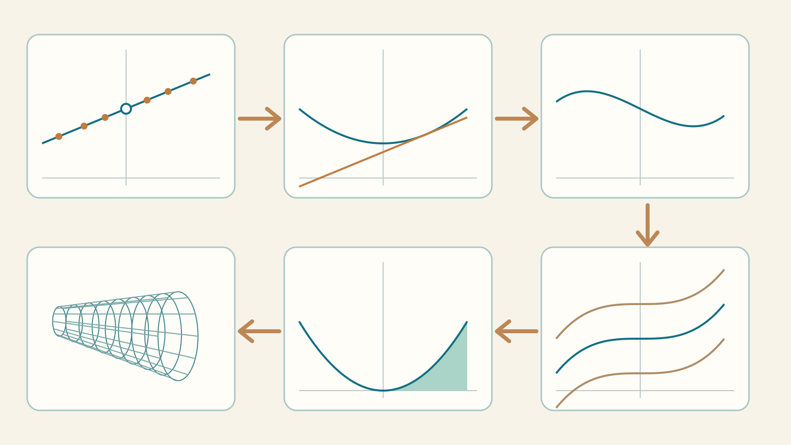
This is the single entrance to the Calculus path. The first block gathers the available foundations; the second organises future extensions without presenting them as published articles. Every available stage links theory and lab, with an explained check before moving on.
Block 1 — Calculus foundations: thirteen stages
Thirteen stages and twelve articles: start with domains, families and transformations before limits. Continuity, sequences, derivatives and function analysis prepare integration; rotations, improper integrals, series, Taylor and first differential equations complete the block. Definite integrals and rotations share an article; sequences and Taylor share a lab. The planned second block is described later in this same index.
Before starting: functions and algebraic tools
Start with real-number arithmetic, integer powers, simple equations and Cartesian coordinates. No prior limits or derivatives are required: the first chapter develops domains, images, families, composition and inverses.
Before simplifying, check nonzero denominators, positive logarithm arguments and nonnegative even-root radicands. For ln(x−1)/√(4−x), simultaneous conditions give 1<x<4. The new opening chapter builds these checks step by step; factoring helps solve inequalities.
Elementary functions: domains, graphs, composition and inverses · Studying a function: understand each step and build its graph · Factoring polynomials: choosing a method, step by step
1. Elementary functions: the foundations
Read domains, images and graphs before using calculus.
Recognise powers, roots, absolute value, reciprocal, exponential, logarithmic and trigonometric functions. Distinguish domains and images, track transformed points, check compositions and build inverses on the correct branch. The lab compares formulas, sets and graphs.
Distinguish √(x²)=|x| from (√x)²=x for x≥0, and inverse from reciprocal.
Read the article · Open the lab
Where is √(3−x) defined and what is its image?
Show the explained check
Require 3−x≥0, hence x≤3. Domain (−∞,3], image [0,+∞). Point (3,0) is included. Horizontal reflection and translation change the domain, not the nonnegative output of the root.
2. Limits and a first look at continuity
Understand what happens near a point or towards infinity.
A limit need not equal the value at the point. Study both sides, excluded points, indeterminate forms and standard limits, then connect limits with continuity. Derivatives come later: do not use l’Hôpital before learning them.
You should distinguish a hole, a jump and infinite behaviour, justifying conclusions beyond a numerical table.
Read the article · Open the lab
Our running example: what is lim(x→1) x²?
Show the explained check
It is 1 because x² is continuous at 1. Here it equals f(1); that is not automatic for every function or point.
3. Continuity and theorems for continuous functions
Move from limits to guarantees about values, zeros and extrema.
Check value, limit and equality at a point; study domains, joins and discontinuities. Intermediate values and Bolzano ensure existence under precise assumptions; Weierstrass ensures attained extrema on closed bounded intervals. The lab compares assumptions, repairs joins and animates bisection.
Distinguish sufficient and necessary criteria, existence and uniqueness, supremum and attained maximum.
Read the article · Open the lab
Why does x² on (−1,2) have a minimum but no maximum?
Show the explained check
0 is attained at x=0; supremum 4 is not attained because x=2 is excluded. Weierstrass does not apply to the open domain, but a minimum can still exist.
4. Sequences: from individual terms to convergence
Understand what happens as the integer index grows without bound.
Move from explicit formulas and recurrences to limits, monotonicity, subsequences and partial sums. Distinguish the sequence of terms from the sequence of sums: terms tending to zero do not guarantee convergence of a series.
Explain why a finite plot does not prove a limit and find a sufficient N for accuracy ε in the covered cases.
Read the article · Open the lab
For aₙ=1/n, which N guarantees |aₙ|<0.05 for every n≥N?
Show the explained check
We need n>20, so choose N=21. Term 20 lies on the boundary of the open band and does not suffice. The limit is 0 regardless of the chosen accuracy.
5. Derivatives: measuring local change
Move from secants to the tangent, and from average to instantaneous change.
Start with the difference quotient and its limit. Only then introduce differentiation rules, the chain rule, non-differentiable points and second derivatives. Rolle’s and the mean value theorem connect local behaviour with an interval.
You should separate height f(a) from slope f′(a), explain why continuity and differentiability are not equivalent, and check theorem hypotheses.
Read the article · Open the lab
For f(x)=x², what is the slope at x=1?
Show the explained check
f′(x)=2x and f′(1)=2. The point is (1,1), and the tangent is y=1+2(x-1)=2x-1. Slope is not the y coordinate.
6. Function analysis: bringing the clues together
Build a justified graph by combining domain, sign, limits and derivatives.
Function analysis now becomes a synthesis: intercepts, symmetry, asymptotes, monotonicity, extrema and concavity must agree. An automatic plot is not enough, nor is merely finding f′=0 or f″=0.
You should explain every branch and distinguish candidates from verified extrema or inflection points.
Read the article · Open the lab
What does the complete analysis of x² tell us?
Show the explained check
Domain ℝ; even and nonnegative; only zero at 0. f′=2x: decreasing until 0 and increasing afterwards. Absolute minimum (0,0). f″=2>0: convex with no inflection points.
7. Indefinite integrals: reconstructing a function
Find F such that F′=f and understand why the answer is a family.
Learn antiderivatives and the constant C, then linearity, substitution, parts and partial fractions. Check by differentiating. Separate domain components may have independent constants.
You should find antiderivatives in the cases studied and distinguish “I have not found a formula” from “no antiderivative exists”.
Read the article · Open the lab
What is the family of antiderivatives of x²?
Show the explained check
F(x)=x³/3+C, since (x³/3+C)′=x². On ℝ all antiderivatives differ by a constant. A condition such as F(1)=2 selects C=5/3.
8. Definite integrals and areas: measuring accumulation
Move from a family of antiderivatives to a number associated with an interval.
Riemann sums introduce accumulation; the fundamental theorem gives F(b)-F(a) under its hypotheses. Distinguish signed integrals, geometric area and area between curves; check orientation, intersections and improper points.
You should explain why an integral can vanish without total area vanishing, and why the final number has no +C.
Read the article · Open the lab
What are the integral and the area below x² from 0 to 1?
Show the explained check
∫₀¹x²dx=[x³/3]₀¹=1/3. Since x²≥0, geometric area is also 1/3. For x on [-1,1], however, the integral is 0 and area is 1.
9. Rotations: distinguishing volume and surface area
Use the correct integral after choosing an axis and a quantity.
Rotating a region produces a solid: disks, washers or shells measure its volume. Rotating a curve generates a surface: its area involves arc length and hence the derivative. Bases are not automatically included in lateral area.
You should identify the axis, radii, possible cavity and units: u³ for volume, u² for surface area.
Read the article · Open the lab
What do we calculate when rotating the region below x² on [0,1] about x?
Show the explained check
Volume is V=π∫₀¹x⁴dx=π/5. The area generated by the curve alone is instead S=2π∫₀¹x²√(1+4x²)dx. To close the solid, its nonzero base adds π to surface area, not to volume.
10. Improper integrals: limits and singularities
Extend integration through limits without confusing convergence and symmetric cancellation.
Study infinite intervals, singular endpoints and interior points by separating all required limits. Use power thresholds and comparisons, control the omitted part and distinguish the ordinary integral from principal value. The lab shows the truncated total and both side contributions.
Explain why ∫₁∞1/x diverges but ∫₁∞1/x² converges, and why ordinary ∫₋₁¹1/x is not 0.
Read the article · Open the lab
What is ∫₁∞dx/x², and what is missing if we stop at R=100?
Show the explained check
The truncation is I(R)=1−1/R, so the limit is 1. At R=100 we get 0.99 and still miss 0.01. A finite truncation is not the complete integral: here the tail formula controls the exact mathematical difference.
11. Numerical and power series
Understand when infinitely many terms have a finite sum and how to control the tail.
Distinguish terms from partial sums, learn tests with their assumptions and separate absolute from conditional convergence. For power series find the radius and test each endpoint: the radius alone does not determine the interval. This chapter prepares Taylor representations of functions.
Explain why aₙ→0 is insufficient, choose an appropriate test and distinguish a remainder bound from actual error.
Read the article · Open the lab
For 1+1/2+1/4+… how many addends guarantee error at most 0.001?
Show the explained check
The sum is 2 and the remainder after N addends is 2¹⁻ᴺ. Ten addends give error 1/512>0.001; eleven give 1/1024<0.001. Eleven suffice, counting the initial 1.
12. Taylor with remainder: approximation with a guarantee
Build a local polynomial and control its possible difference from the function.
Use derivatives at centre a to build Tₙ. The Lagrange remainder relates error to a bound on derivative n+1 over the whole segment. Distinguish the finite formula, Peano remainder and infinite series: increasing the order does not always guarantee convergence to the function.
Distinguish actual error from a bound, check the domain and assumptions, and seek an order that certifies a tolerance.
Read the article · Open the lab
At centre 0 and order 3, what approximates exp(0.2), and what is its remainder bound?
Show the explained check
T₃(0.2)=1+0.2+0.2²/2+0.2³/6≈1.221333333. On [0,0.2], M=exp(0.2), so |R₃|≤M·0.2⁴/24≈0.000081427. Actual error is about 0.000069425, not equal to the bound.
13. First differential equations: describing evolution
Find a function from a rate law and an initial value.
Distinguish an equation from an initial-value problem. Start with antiderivatives, separate variables without losing equilibria, use integrating factors for linear equations and build exponential, cooling and logistic models. The lab compares slope fields, solutions, Euler and Heun, checking domain, uniqueness and stability.
Verify a solution and distinguish numerical error, model limits and nonuniqueness.
Read the article · Open the lab
Which function solves y′=2t, y(0)=0?
Show the explained check
Integration gives y=t²+C. The initial value sets C=0, hence y=t². Its derivative is 2t and y(0)=0, verifying both conditions. Heun reproduces the nodal values here in exact arithmetic, whereas Euler introduces a difference.
One function, different questions
Following x² shows why these operations must not be confused. Each stage links to the matching lab example; try before revealing the explained check.
| Question | Answer for x² |
|---|---|
| The graph of x² | D=ℝ; Im=[0,+∞); f(−x)=f(x) |
| Behaviour near 1 | lim(x→1)x²=1 |
| Continuity of x² | lim(x→a)x²=a²=f(a); min[−1,2]=0, max[−1,2]=4 |
| Approach through integer indices | aₙ=(1+1/n)² → 1 |
| Slope at 1 | f′(1)=2 |
| Graph shape | Minimum at (0,0), convexity, no inflection |
| Reconstruction from f=x² | F=x³/3+C |
| Accumulation on [0,1] | ∫₀¹x²dx=1/3 |
| Volume of rotation about x | V=π/5 |
| Improper tail for x² | ∫₁ᴿx²dx=(R³−1)/3 → +∞ |
| Power series for x² | 0+0x+1x²+0x³+… = x²; R=∞ |
| Taylor centred at 1 | T₂(x)=1+2(x−1)+(x−1)²=x²; R₂=0 |
| An equation for x² | y′=2t, y(0)=0 ⇒ y=t² |
The bridge to algorithms: numerical approximations
Bisection and Newton find zeros; midpoint, trapezoidal, Simpson and Monte Carlo methods estimate integrals. The Taylor introduction in Mathematics → Algorithms remains a numerical application; the Calculus chapter now develops coefficients, assumptions, Lagrange remainder and convergence, with its own lab. A small difference between refinements is not by itself a guaranteed error bound.
How to study and review
- Read the problem motivating a stage and write down what you need to find.
- Try an example on paper, specifying domain, assumptions and result type.
- Use the lab to explore and compare, not to replace a proof with a picture.
- Reveal the solution after your attempt and identify the source of any error.
- Move on when you can explain the result, not merely apply a formula.
Use the stage index to review a specific problem. For complete study, follow the suggested order and return to function analysis after learning limits and derivatives.
Block 2 — Planned extensions
These are future developments, not links to published chapters. We keep one index: each extension will have an article and lab when ready.
- Second-order differential equations
Current coverage: First order is in the foundations.
Useful next step: Oscillations, springs and damping with animations.
- Systems of differential equations
Current coverage: Single equations have been introduced.
Useful next step: Two linked quantities, trajectories and equilibria.
- Uniform continuity and Heine–Cantor
Current coverage: Pointwise continuity, Bolzano and Weierstrass are available.
Useful next step: Control a whole function with one choice of δ.
- Function series and uniform convergence
Current coverage: Numerical and power series are in block one.
Useful next step: When limits, derivatives and integrals may be interchanged.
- Fourier series
Current coverage: Sine and cosine are now in the foundations.
Useful next step: Reconstruct shapes and signals by adding waves.
The goal: choosing reasoning, not just a formula
You should recognise whether a problem concerns approach, change, reconstruction or accumulation, then select a tool and justify its conditions. Return to this index whenever a step is unclear.