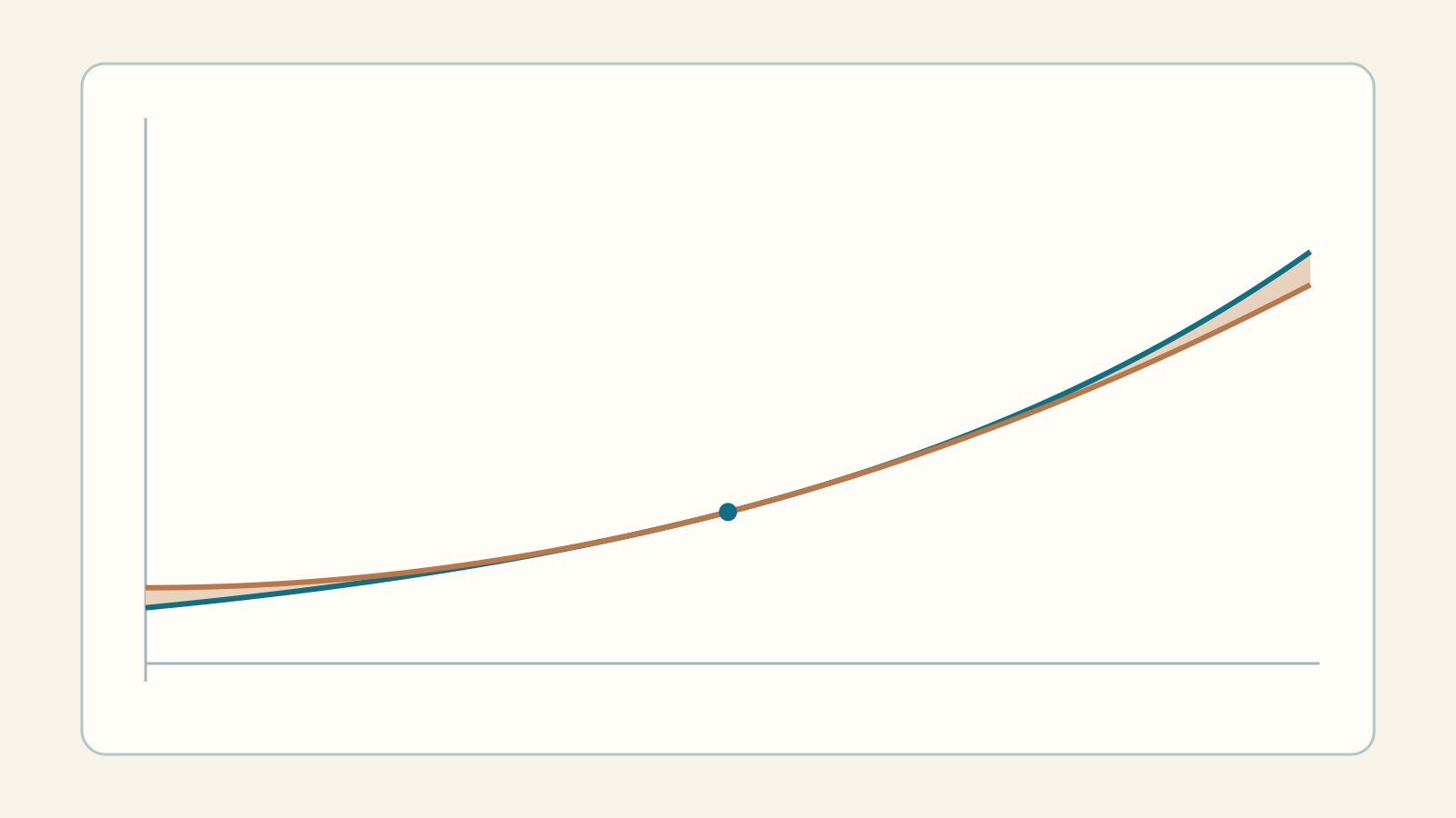
Saying “approximately” is not enough: how wrong could we be? Taylor builds a polynomial from derivatives at one point and accompanies it with a remainder. The key question is not how many terms we can write, but where and with what accuracy we may use them.
Sequences and Taylor lab · Learning-path index
1. From the tangent to a polynomial
Near centre a, T₀(x)=f(a) matches the value; T₁(x)=f(a)+f′(a)(x−a) also matches the slope. Matching the second derivative adds f″(a)(x−a)²/2. We are not interpolating data at different points or fitting a regression: value and derivatives are imposed at one point.
The centre a and evaluation point x need not coincide. Quantity h=x−a measures the distance from the centre.
2. Why factorials appear
Write P(x)=c₀+c₁(x−a)+…+cₙ(x−a)ⁿ. Evaluating at a gives P(a)=c₀; differentiating once gives P′(a)=c₁. After k derivatives P⁽ᵏ⁾(a)=k!cₖ: lower terms disappear and higher terms still contain x−a.
cₖ=f⁽ᵏ⁾(a)/k!
Tₙ(x)=Σₖ₌₀ⁿ [f⁽ᵏ⁾(a)/k!](x−a)ᵏ
0!=1. Degree is at most n: some coefficients can vanish. Centre a=0 gives Maclaurin. For sin(x), T₂=T₁=x; maximum order 2 need not mean actual degree 2.
3. Finite formula and Lagrange remainder
A convenient sufficient condition is that f has n+1 continuous derivatives on an open interval containing the whole segment from a to x. Then, for x≠a, some ξ strictly between a and x satisfies:
f(x)=Tₙ(x)+Rₙ(x)
Rₙ(x)=f⁽ⁿ⁺¹⁾(ξ)(x−a)ⁿ⁺¹/(n+1)!
We call the remainder after Tₙ Rₙ; other texts call it Rₙ₊₁. ξ exists but is usually unknown. We may not arbitrarily replace it with a or x. At x=a the remainder is 0. The finite formula does not require an infinite series to converge.
4. From identity to a guaranteed bound
If |f⁽ⁿ⁺¹⁾(t)|≤M throughout the segment from a to x, then:
|Rₙ(x)|≤M|x−a|ⁿ⁺¹/(n+1)!
M bounds the derivative over the entire segment, not a few sampled points. Actual error is |f(x)−Tₙ(x)|; the bound may be much larger. A bound exceeding tolerance fails to certify accuracy but does not prove the approximation is poor.
Under the same assumptions, repeated integration by parts gives Rₙ(x)=(1/n!)∫ₐˣ f⁽ⁿ⁺¹⁾(t)(x−t)ⁿdt. Taking absolute values and integrating M|x−t|ⁿ yields the bound. This integral form connects Taylor to definite integration.
5. Three worked examples with error control
e0.2, centre 0, order 3. Every derivative of eˣ is eˣ. T₃(0.2)=1+0.2+0.2²/2+0.2³/6=1.221333333… . On [0,0.2], M=e0.2. The remainder is at most e0.2·0.2⁴/24≈0.000081427. Actual error is about 0.000069425, below the bound.
ln(1.5), centre 0 for f(x)=ln(1+x), order 4. T₄(0.5)=0.5−0.5²/2+0.5³/3−0.5⁴/4≈0.401041667. The fifth derivative is 24/(1+x)⁵, so M=24 on [0,0.5]. The bound is 0.5⁵/5=0.00625; actual error is about 0.004423441.
√1.21, centre 0 for √(1+x), order 2. T₂(0.21)=1+0.21/2−0.21²/8=1.0994875. The third derivative is 3/[8(1+x)⁵ᐟ²], so M=3/8. The bound is 0.0005788125; the exact value is 1.1 and the error 0.0005125.
6. Choosing the order and centre
For sin(0.1), T₃=x−x³/6. With M=1 the order-3 bound is 0.1⁴/24. But T₄=T₃ because the x⁴ coefficient vanishes: applying the theorem at order 4 gives the sharper bound 0.1⁵/120≈8.33·10⁻⁸ without changing the polynomial.
To estimate e1.1 we may centre at a=1: T₂(1.1)=e[1+0.1+0.1²/2]. The relevant h is 0.1, not x=1.1. A nearby centre can need fewer terms if its derivatives are known.
For tolerance δ seek an order with M|h|ⁿ⁺¹/(n+1)!≤δ. The lab’s “Find order” searches 0 to 30: the first order certified by this bound need not be the minimum actual degree giving acceptable error.
7. Finite formula, series and validity interval
For fixed x, Tₙ(x)→f(x) exactly when Rₙ(x)→0 as n→∞. Having all derivatives is insufficient. The series for eˣ, sin(x), cos(x) represent their functions at every real x.
At centre 0, 1/(1−x)=1+x+x²+… only for |x|<1. At x=−1 the function equals 1/2 but partial sums oscillate; at x=1 it is undefined. The exact finite remainder is Rₙ=xⁿ⁺¹/(1−x), making the distinction verifiable without a graph.
ln(1+x)=x−x²/2+x³/3−… represents the function for −1<x≤1; at x=1 convergence is slower and needs a separate endpoint argument. The series of √(1+x) at 0 represents it at both endpoints −1 and 1 as well. The lab excludes x=−1 for root and logarithm: the continuous-derivative bound on the segment is unavailable there.
For logarithm and root centred at a>−1 the radius is 1+a; for 1/(1−x) it is |1−a|. Outside that radius a finite remainder formula can still be valid on the same domain branch, but increasing n need not converge to the function. Radius inequalities alone do not settle endpoints.
8. Peano remainder: a different limit
If f is Cⁿ near a, then f(x)=Tₙ(x)+o((x−a)ⁿ) as x→a. This means Rₙ(x)/(x−a)ⁿ→0: n is fixed while x approaches the centre. It is not the limit n→∞ at fixed x, nor does it by itself provide a numerical M to certify error at a finite distance.
For example eˣ=1+x+x²/2+o(x²) gives limₓ→₀(eˣ−1−x)/x²=1/2. Keeping only 1+x would miss the first nonzero term needed.
9. Having all derivatives is not enough
Define f(0)=0 and f(x)=e^(−1/x²) for x≠0. All derivatives at 0 vanish. Away from 0 each derivative is a polynomial in 1/x times e^(−1/x²), which tends to 0 faster than any power; the same applies to difference quotients at 0.
Every Tₙ is zero. The zero series converges everywhere but represents f only at 0: f is positive elsewhere. The lab treats this case separately: actual error is shown, but no remainder bound or certified order is computed. Lagrange’s theorem has not failed: the remainders do not tend to 0 as n→∞.
10. Experiments and lab limitations
Choose one of seven functions, centre a, evaluation point x and order n. The plots compare function and polynomial; a table lists cₖ and cₖ(x−a)ᵏ. Play increases the order from 0 to 30. The panel distinguishes function value, approximation, numerical error and Lagrange bound, with M calculated analytically on the segment.
Try 1/(1−x) at a=0, first x=0.5, then x=−1. For eˣ move the centre from 0 to 1. The flat case keeps a=0. Segments crossing poles or domain boundaries are rejected. Numerical values are rounded: guarantees concern the mathematical polynomial, not certified interval arithmetic on the computer.
Exercises: try before revealing
1. Build T₃ of eˣ at 0.
2. Why is c₂=f″(a)/2, not f″(a)?
Show the explained answer
The second derivative of c₂(x−a)² is 2c₂: set 2c₂=f″(a) and divide by 2!=2.
3. Estimate sin(0.1) with T₄ at 0.
4. Does an error bound of 0.01 prove the error equals 0.01?
Show the explained answer
No: it guarantees only |Rₙ|≤0.01. Actual error may be much smaller.
5. At centre 0, does Tₙ of 1/(1−x) converge at x=−1?
Show the explained answer
No: 1−1+1−… has sums 1,0,1,0,… . The function equals 1/2 but the polynomials do not converge to it.
6. Find limₓ→₀(eˣ−1−x)/x².
Show the explained answer
eˣ−1−x=x²/2+o(x²); dividing by x² gives limit 1/2.
7. Do all derivatives vanishing at 0 imply f is identically zero?
Show the explained answer
No: f(0)=0, f(x)=e^(−1/x²) for x≠0 is positive away from 0 and every derivative vanishes at 0.
8. For ln(1+x), can the Lagrange bound centred at 0 include x=−1?
Show the explained answer
No: ln(0) is undefined and the derivatives are not continuous on that segment. A computable polynomial is not enough.
Sequences: from the first terms to convergence · Review limits · Review derivatives