After limits, we ask a new question: how rapidly does a quantity change at a particular instant or point? A derivative arises from a limit, but also becomes a function to study. We build its meaning before introducing the rules, then connect calculations, graphs and applications.
What does a derivative measure?
If s(t) is a position in metres and t is time in seconds, [s(t+h)-s(t)]/h measures average velocity over the interval. To find instantaneous velocity, let h approach zero. If a function describes cost in euros against production quantity, its derivative measures euros per unit of product.
A derivative is a local rate of change: not the height of the graph. A function can be positive yet decreasing, with a negative derivative. Its units are output units divided by input units.
The difference quotient and the secant line
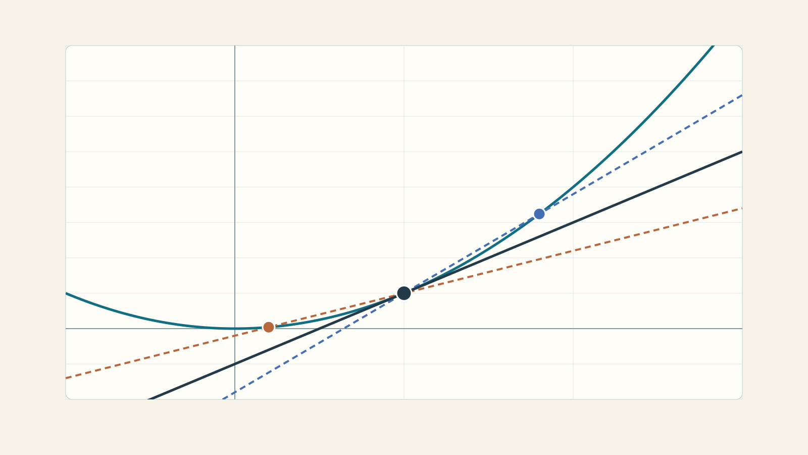
Fix P=(a,f(a)) and a nearby point Q=(a+h,f(a+h)), with h≠0. The horizontal increment is h and the vertical increment is f(a+h)-f(a). The secant slope is:
Q(h) = [f(a+h)-f(a)]/h
h may be positive or negative. Do not change only the denominator’s sign: a negative h changes a+h as well. The anchor a and nearby inputs used must belong to the domain.
The derivative is a limit, not division by zero
The ordinary derivative at an interior point a is the finite limit:
f′(a) = lim(h→0) [f(a+h)-f(a)]/h
Calculate the quotient for h≠0, then study its limit. Substituting h=0 and obtaining 0/0 is not an answer. For the derivative to exist, the left-hand and right-hand limits of the difference quotient must coincide and be finite.
f′(a) denotes a number, whereas f′(x) denotes the derivative function. The notations y′ and dy/dx express the same concept; dy/dx does not justify always treating its symbols as an ordinary fraction.
A complete calculation from the definition: f(x)=x²
We have f(a+h)=(a+h)²=a²+2ah+h² and f(a)=a². Thus:
Q(h)=[a²+2ah+h²-a²]/h=(2ah+h²)/h=2a+h, for h≠0.
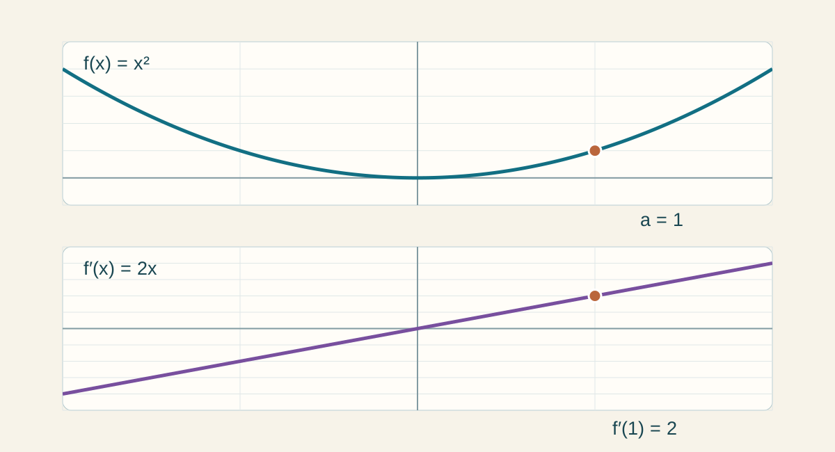
Letting h→0 gives f′(a)=2a, hence f′(x)=2x. At a=1 the derivative is 2; h=0.1 gives a quotient of 2.1 and h=-0.1 gives 1.9. Both approach 2 from opposite sides.
For a constant c the numerator c-c is 0, so the derivative is 0. For a line mx+q the difference quotient is always m, so its derivative is m.
The tangent equation and local approximation
If f is differentiable at a, its tangent passes through (a,f(a)) with slope f′(a):
y = f(a) + f′(a)(x-a)
For x² at a=1: y=1+2(x-1)=2x-1. A secant instead has slope Q(h), still dependent on h. A tangent may cross the graph; it need not touch it at only one point.
For small increments, f(a+h)≈f(a)+f′(a)h. For √x at a=4: √(4.04)≈2+(1/4)·0.04=2.01. This is an approximation, not an exact equality; differentiability alone ensures an error small compared with h, not a generally zero error.
Differentiability and continuity: a one-way implication
If f is differentiable at a, it is continuous there. Indeed, for h≠0, f(a+h)-f(a)=Q(h)·h; if Q(h) approaches a finite number, the product tends to 0.
The converse is false. |x| is continuous at zero, but its difference quotients are -1 on the left and 1 on the right: there is no unique derivative. Continuity is necessary, not sufficient.
If the point is missing, as x=1 is for (x²-1)/(x-1), we cannot even form a quotient anchored at f(1). The original function has no derivative there, although its derivative elsewhere is 1.
Corners, cusps, vertical tangents and endpoints
|x|at zero: two finite but different one-sided slopes, a corner.|x|^(2/3)at zero: quotients tend to -∞ on the left and +∞ on the right, a cusp with vertical one-sided tangents; no finite derivative.cbrt(x)at zero: quotients tend to +∞ on both sides, a vertical tangent x=0 but no finite ordinary derivative.√xat zero: the domain only permits a right-hand quotient, tending to +∞. This is one-sided endpoint behaviour, not an ordinary two-sided derivative.- A function with a jump is not continuous at that point, so it cannot be differentiable there.
The symmetric quotient [f(a+h)-f(a-h)]/(2h) does not replace the definition: for |x| at zero it is always 0, although the derivative does not exist.
Basic derivatives and their domains
| Function | Derivative | Conditions |
|---|---|---|
| c | 0 | c constant |
| xⁿ | nx^(n-1) | For positive integer n, on ℝ |
| x^α | αx^(α-1) | For real α, certainly on x>0; other cases require the appropriate domain |
| 1/x | -1/x² | x≠0 |
| √x | 1/(2√x) | x>0 |
| eˣ | eˣ | ℝ |
| bˣ | bˣ ln b | b>0, b≠1 |
| ln x | 1/x | x>0 |
| log_b x | 1/(x ln b) | x>0, b>0, b≠1 |
| sin x | cos x | Radians |
| cos x | -sin x | Radians |
| tan x | 1/cos²x | cos x≠0, radians |
The table does not remove exclusions from the original function. For example, (ln|x|)′=1/x for x≠0, whereas ln x is not defined for negative x.
Sums, differences and constant factors
Where the functions involved are differentiable, (u+v)′=u′+v′, (u-v)′=u′-v′, and (cu)′=cu′ for constant c.
Example: f(x)=3x⁴-2x²+7x-5. Differentiate term by term: f′(x)=12x³-4x+7. The -5 term disappears because it is constant; 7x gives 7, not 0.
Simplify when permitted before applying many rules: x·x=x². Keep the original domain when simplifying a fraction.
Products and quotients: not separate differentiation
(uv)′=u′v+uv′, not u′v′. For x sin x, f′=1·sin x+x·cos x.
(u/v)′=(u′v-uv′)/v², with v≠0. For (x²+1)/(x-1):
f′=[2x(x-1)-(x²+1)]/(x-1)²=(x²-2x-1)/(x-1)²=1-2/(x-1)², for x≠1. Watch the subtraction order and the squared denominator.
Compositions: the chain rule
For f(x)=g(u(x)), differentiate the outer function at the inner value and multiply by the derivative of the inner function:
f′(x)=g′(u(x))·u′(x)
For (3x+1)⁴: outer u⁴ → 4u³; inner 3x+1 → 3. Thus f′=4(3x+1)³·3=12(3x+1)³. For sin(x²) we obtain 2x cos(x²); for ln(x²+1), 2x/(x²+1).
Chains combine with products and quotients. For x²e^(3x), f′=2xe^(3x)+3x²e^(3x). Omitting the inner factor is a frequent mistake.
A further step: implicit and logarithmic differentiation
If x²+y²=25 locally defines y as a differentiable function of x, differentiate y using the chain rule too: 2x+2y·y′=0, hence y′=-x/y where y≠0. At y=0 this formula gives no finite slope, requiring separate analysis.
For y=x^x, with x>0, take logarithms: ln y=x ln x. Differentiating gives y′/y=ln x+1, so y′=x^x(ln x+1). A constant-exponent power rule is insufficient when the exponent also depends on x.
Derivative signs, extrema and optimisation
On an interval, f′>0 implies increase and f′<0 decrease. Do not join intervals across an excluded point. Points with f′=0 are candidates, not automatic maxima or minima: x³ increases through zero.
A sign change from + to - indicates a local maximum; from - to + a local minimum. Check non-differentiable points and included endpoints too. On a closed interval, compare all candidates with its endpoints when optimising.
Example: a rectangle with perimeter 20. One side x gives the other as 10-x, so A(x)=x(10-x) for 0<x<10. A′=10-2x is positive before 5 and negative after. The maximum area is A(5)=25, attained by a 5×5 square.
The second derivative: how slope changes
The second derivative f″ is the derivative of f′. Where f″>0, slope increases and the graph is concave up; where f″<0, slope decreases and it is concave down. For position s(t), s′ is velocity and s″ acceleration: metres per second and metres per second squared.
An inflection requires an actual change of concavity at a point of the graph. x⁴ has f″=12x², zero at the origin but positive on both sides: no inflection. x³ has f″=6x, which changes sign, giving an inflection at zero.
The test f′(a)=0 with f″(a)>0 gives a local minimum; with f″(a)<0, a local maximum, under the usual regularity assumptions. If f″(a)=0, the test is inconclusive.
Rolle and the mean value theorem: average and instantaneous change
Rolle: if f is continuous on [u,v], differentiable on (u,v), and f(u)=f(v), some interior c satisfies f′(c)=0. For f(x)=x² on [-1,1], c=0.
The mean value theorem: with continuity on [u,v] and differentiability on (u,v), an interior c satisfies f′(c)=[f(v)-f(u)]/(v-u). A tangent is parallel to the endpoint secant. For x² on [0,2], the average slope is 2 and f′(1)=2.
Assumptions matter: |x| on [-1,1] has equal endpoint values but is not differentiable at zero and has no point with derivative zero. We cannot ignore the corner and apply Rolle.
Back to limits: L’Hôpital with care
For 0/0 or ∞/∞ forms, under the theorem’s assumptions, we may study the quotient of derivatives. In a usual version, f and g are differentiable in a punctured neighbourhood, g′≠0, and the limit of f′/g′ exists, finite or infinite. Other domain and quotient conditions must also hold.
lim(x→0)(e^x-1)/x=lim(x→0)e^x/1=1, provided the exponential derivative has already been established independently. Do not use a rule to prove the limit from which that same rule was derived.
This is not the quotient differentiation rule: we compare limits of ratios, not assert (f/g)′=f′/g′. Other indeterminate forms first need transforming; when simple factoring suffices, it is often clearer.
Symbolic differentiation and numerical estimation are different
A formula for f′ comes from rules and their conditions. A finite difference uses a small but non-zero h and is an estimate. If h is too large, its quotient stays far from the derivative; if too small, subtracting nearly equal values loses digits.
Guided cases use stable equivalent quotients where possible: for x², Q(h)=2a+h; for eˣ, Q(h)=e^a·expm1(h)/h. This does not change their mathematical meaning. Free input evaluates the expression and explains calculation limits, without automatically certifying differentiability.
An unevaluable derivative formula is not by itself proof of non-differentiability: simplification or separate difference-quotient analysis may be needed. A graph is sampled too, not a proof.
How to explore the laboratory
Choose one of seventeen cases or enter a function. You can change a even in guided cases; the selector shows positive h, negative h or both. The slider reduces |h| from 1 to 10⁻⁶. Play, Pause and One step show the secants converging.
The first graph compares f, secants and the tangent when justified; the second shows f′ and optionally f″. Enable close-up zoom and compare the quotient tables, including the symmetric quotient. Explanations clearly distinguish non-regular cases.
Guided piecewise definitions are preconfigured. Free input uses expressions in x, radians and decimal points. General conclusions require reasoning, not a few screen values.
Return to the meaning of a limit · Open the limits laboratory
Connect to function analysis · Open function analysis
Sixteen exercises: open solutions after trying
1. x^2
Find the derivative at 2 from the definition and the tangent.
Show the explained solution
Q(h)=4+h→4. The point is (2,4), so y=4+4(x-2)=4x-4.
2. 3*x^4-2*x^2+7*x-5
Differentiate term by term.
Show the explained solution
f′=12x³-4x+7. At zero the slope is 7 and f(0)=-5, giving tangent y=-5+7x.
3. x*sin(x)
Apply the product rule.
Show the explained solution
f′=sin x+x cos x. At zero, f′=0 and f=0, giving horizontal tangent y=0.
4. (x^2+1)/(x-1)
Differentiate the quotient while preserving the domain.
Show the explained solution
f′=[2x(x-1)-(x²+1)]/(x-1)²=1-2/(x-1)², x≠1. At zero f=-1 and f′=-1, so y=-1-x.
5. (3*x+1)^4
Identify the outer and inner functions.
Show the explained solution
Outer u⁴, inner 3x+1: f′=4(3x+1)³·3=12(3x+1)³. At zero the slope is 12.
6. ln(x^2+1)
Use the chain rule for the logarithm.
Show the explained solution
Its argument is always positive. f′=2x/(x²+1), equal to 1 at x=1. The tangent is y=ln 2+(x-1).
7. sqrt(1+x^2)
Differentiate the composite square root.
Show the explained solution
f′=[1/(2√(1+x²))]·2x=x/√(1+x²). At zero the slope is 0 and f=1, giving y=1.
8. x^2*exp(3*x)
Combine product and chain rules.
Show the explained solution
f′=2xe^(3x)+3x²e^(3x)=e^(3x)(2x+3x²). At 1 this is 5e³.
9. abs(x)
Does a zero symmetric quotient prove differentiability?
Show the explained solution
No. The left and right difference quotients are -1 and 1, so no derivative exists. The symmetric quotient is 0 but is not the limit required by the definition.
10. cbrt(x)
Describe the slope at zero.
Show the explained solution
Q(h)=cbrt(h)/h=1/|h|^(2/3)→+∞ from both sides. The tangent is vertical, x=0; no finite ordinary derivative exists.
11. sqrt(x)
Why does the domain endpoint need care?
Show the explained solution
There are no real left-hand samples at zero. On the right Q(h)=1/√h→+∞. This is one-sided endpoint behaviour, not a finite two-sided derivative.
12. x^3
Does a zero derivative imply an extremum?
Show the explained solution
No. f′=3x²≥0 and the function increases through zero. f″=6x changes sign, giving an inflection with a horizontal tangent.
13. x^4
Apply the second derivative test at zero.
Show the explained solution
f′(0)=0 and f″(0)=0, so the test is inconclusive. The signs of f′=4x³ give a minimum. f″=12x² does not change sign, so there is no inflection.
14. x*(10-x)
Maximise the area of a rectangle with perimeter 20.
Show the explained solution
For 0<x<10, A′=10-2x changes from positive to negative at 5. A(5)=25 is the maximum; both sides are 5.
15. x^x
Differentiate using logarithms, for x>0.
Show the explained solution
From ln y=x ln x, y′/y=ln x+1. Thus y′=x^x(ln x+1), equal to 1 at x=1.
16. x^2
Find the mean-value point for x² on [0,2].
Show the explained solution
The function is continuous on [0,2] and differentiable on (0,2). Average slope is (4-0)/(2-0)=2. Solving 2c=2 gives c=1, inside the interval.