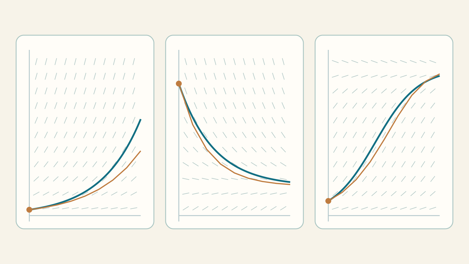
So far we have differentiated known functions or recovered antiderivatives. Now we know a law connecting a quantity to its rate of change and seek a function obeying that law. This moves from calculating a curve to building a dynamic model. We start with first-order equations, worked examples and explicit limitations.
First differential equations lab · Learning-path index
1. The unknown is a function
In 2x+3=7 we seek a number. In y′(t)=F(t,y(t)) we seek a differentiable function on an interval: its derivative must equal the right-hand side at every point. t is the independent variable, y the evolving quantity and y′ its instantaneous rate of change. Verify a solution by differentiating and substituting into the equation, not by checking a few values.
The order is the highest derivative present: y′=2t is first order, y″+y=0 second order. Here we study first-order ordinary differential equations with one independent variable. Partial differential equations and systems are later extensions.
2. A family and an initial condition
From y′=2t we get y=t²+C: every member has the required derivative. The condition y(0)=3 selects C=3, hence y(t)=t²+3. Check y′=2t and y(0)=3. An equation together with an initial value is an initial-value problem. With y(t₀)=y₀, the same equation gives y=t²+y₀−t₀².
In integral form, y′=F(t,y), y(t₀)=y₀ is equivalent, under the usual continuity assumptions, to y(t)=y₀+∫t₀tF(s,y(s))ds. Total change accumulates the rates. This is not yet explicit because y also appears inside the integral.
3. Reading a slope field
At each point (t,y), F(t,y) gives the slope a solution must have there. A short segment with that inclination produces a slope field. For y′=−y, segments slope down above the axis, are horizontal at y=0 and slope up below it. Curves approach 0 forwards in time.
The field is not a solution: it indicates local tangents. An initial value fixes a point to pass through. In the lab, touch the graph to read F(t,y) and inspect a tangent segment; this does not move the initial value, which has its own input.
4. Separating variables without losing solutions
If y′=g(t)h(y), first find equilibria h(y)=0. Where h(y)≠0, write y′/h(y)=g(t) and integrate: ∫dy/h(y)=∫g(t)dt+C. This follows from the chain rule, not from treating dy and dt as independent numbers in every setting. The resulting relation may remain implicit.
Example: y′=2t(y+1). First find the constant solution y=−1. For y≠−1, integration gives ln|y+1|=t²+C. Exponentiating and absorbing sign and constant gives y=Cet²−1; C=0 also recovers the equilibrium. With y(0)=2, C=3. Dividing immediately by y+1 and forgetting its zero would lose a solution.
5. Growth, decay and characteristic times
“Growth rate proportional to the present amount” becomes y′=ky. For y≠0, y′/y=k gives ln|y|=kt+C and y=Cekt. Include equilibrium y=0. With y(0)=y₀ we obtain y(t)=y₀ekt. For y₀>0, k>0 gives growth, k<0 decay; k=0 keeps the amount constant.
Example: y₀=5 and k=0.2 per hour. After 5 hours, y=5e≈13.5914. Doubling time is ln 2/k≈3.4657 hours. For y′=−λy with λ>0, half-life is ln 2/λ. Both parameters have inverse-time units: kt must be dimensionless. k=0.2 does not mean multiplying by 1.2 each hour: the continuous one-hour factor is e0.2.
6. Cooling towards an ambient temperature
With constant ambient temperature A and rate proportional to the temperature difference, the model is y′=−k(y−A), k>0. Set z=y−A, so z′=−kz and y(t)=A+(y₀−A)e−kt. Above A the object cools, below A it warms; y=A is a stable equilibrium.
A drink starts at 80 °C in a 20 °C room. Choose k=(ln 2)/10 per minute: after 10 minutes the difference halves and y(10)=20+60/2=50 °C; after 20 minutes y(20)=35 °C. It is the difference from ambient, not the body temperature value, that halves. The model assumes a constant environment and coefficient: a mathematical curve does not replace measurements and experimental checks.
7. Growth with a limit: the logistic model
Exponential growth ignores finite resources. Introduce capacity K>0: y′=ry(1−y/K), r>0. Equilibria are y=0 and y=K. Growth is positive for 0<y<K and negative for y>K. Separation uses K/[y(K−y)]=1/y+1/(K−y), giving ln|y|−ln|K−y|=rt+C.
For y₀>0 the forward solution is y(t)=K/[1+(K/y₀−1)e−rt], including y₀=K; y₀=0 separately gives y=0. With K=10, r=1, y₀=2: y=10/(1+4e−t) and y(ln 4)=5. For 0<y₀<K, the largest growth rate occurs at y=K/2 because y′=rK/4−(r/K)(y−K/2)². Not every real population follows a logistic law.
8. Linear equations and integrating factors
A first-order linear equation has form y′+a(t)y=b(t), without terms such as y² or yy′. With continuous a and b on an interval, choose nonzero μ(t)=exp(∫a(t)dt). Since μ′=aμ, multiplication gives μy′+μay=μb, hence (μy)′=μb. Integrating and dividing by μ gives y=[C+∫μb dt]/μ. One antiderivative suffices for μ: its multiplicative constant is irrelevant.
Worked example: y′+2y=4t, y(0)=1. μ=e2t, so (e2ty)′=4te2t. Integration by parts gives ∫4te2tdt=e2t(2t−1)+C. Thus y=2t−1+Ce−2t. The initial value gives 1=−1+C, C=2, hence y=2t−1+2e−2t. Check: y′=2−4e−2t; adding 2y leaves 4t.
9. Existence, uniqueness and the solution interval
An initial value does not always select one solution. A local sufficient condition is that F is continuous in an open rectangle around (t₀,y₀) and locally Lipschitz in y uniformly in t. Lipschitz means a common constant L controls |F(t,y₁)−F(t,y₂)|≤L|y₁−y₂| in a suitable neighbourhood. A continuous partial derivative ∂F/∂y there is an easy sufficient check. This gives a unique solution on a sufficiently small interval, not necessarily for all time.
Unique but not global: y′=y², y(0)=1 gives y=1/(1−t), with maximal interval containing 0 equal to (−∞,1). It diverges as t→1⁻. The same rational expression for t>1 does not extend the solution through the pole.
Nonunique: y′=2√|y|, y(0)=0 admits y=0 and, for each τ≥0, y=0 up to τ and y=(t−τ)² afterwards, for t≥0. Both one-sided derivatives at the join are 0, so these really are solutions. F is continuous but not locally Lipschitz at y=0. The lab displays a curve selected by τ, not “the unique solution”.
10. Euler: stepping along the tangent
With tₙ=t₀+nh and h>0, explicit Euler uses the current slope for the whole step: yₙ₊₁=yₙ+hF(tₙ,yₙ). For y′=y, y(0)=1 and h=0.5: y₁=1+0.5×1=1.5; y₂=1.5+0.5×1.5=2.25. At t=1 the exact solution is e≈2.71828, giving absolute error about 0.46828.
With enough regularity, on a fixed interval and under the required stability conditions, global error is O(h): halving h tends asymptotically to halve it. Two numerical trials alone do not certify an error bound. For y′=−ky, Euler gives yₙ₊₁=(1−kh)yₙ: asymptotic stability requires |1−kh|<1, or 0<kh<2. Preserving nonnegative positive-data trajectories additionally requires kh≤1. Numerical oscillations need not exist in the model.
11. Heun: prediction and correction
Explicit Heun evaluates two slopes: k₁=F(tₙ,yₙ); predictor ỹ=yₙ+hk₁; then k₂=F(tₙ+h,ỹ). Correct with their mean: yₙ₊₁=yₙ+h(k₁+k₂)/2. For y′=y, y₀=1, h=0.5: k₁=1, ỹ=1.5, k₂=1.5, y₁=1.625. The next step gives y₂=2.640625, closer to e than Euler.
This is a second-order explicit Runge–Kutta method: in regular conditions global error is O(h²). It is not the implicit trapezoidal method, which evaluates F at the unknown corrected value. Heun is not always better for every step and problem: stability and domain matter. For y′=2√|y| with zero initial value, both methods stay exactly at zero: a valid solution even when the chosen τ-curve differs.
12. A practical workflow and the lab
- Define quantities, independent variable and units.
- Translate the law into an equation and specify initial data.
- Classify: direct integration, separable, linear or outside scope.
- Check equilibria and divisions; solve and impose the data.
- Find the validity interval; verify derivative and initial value.
- Compare with the physical model before comparing numerical approximations.
Choose a lab case, edit parameters and press Explore. The slider, Step and Play advance numerical construction while the reference solution remains visible. Halve the step to compare nodal errors. The table shows values and differences; the detail explains the last step. These are seven guided families, not a universal symbolic solver. A finite grid proves neither existence, uniqueness nor convergence.
Exercises: try before revealing
1. Solve y′=2t, y(0)=−2.
Show the explained answer
Integration gives y=t²+C; the data give C=−2. Thus y=t²−2 on ℝ. Its derivative is 2t and initial value −2.
2. y′=−0.5y, y(0)=8: value after ln 4?
Show the explained answer
y=8e^(−t/2). At t=ln 4, e^(−ln4/2)=1/2, hence y=4. Half-life is ln2/0.5=ln4.
3. Ambient 20, y₀=80: when is y=50?
Show the explained answer
From 50=20+60e^(−kt), e^(−kt)=1/2 and t=ln2/k. If k=ln2/10, t=10 minutes. The temperature excess halves, not 80.
4. Logistic K=10, r=1, y₀=2: when is y=5?
Show the explained answer
5=10/(1+4e^(−t)) gives 1+4e^(−t)=2, e^(−t)=1/4 and t=ln4. This trajectory has its greatest growth rate there.
5. Which solution is lost by dividing y′=2t(y+1) by y+1?
Show the explained answer
y=−1. Its derivative is zero and the right-hand side vanishes. Check zeros before dividing; the final family Ce^(t²)−1 recovers it at C=0.
6. Solve y′+2y=4t, y(0)=1.
Show the explained answer
μ=e^(2t). Integrating (μy)′=4tμ gives y=2t−1+Ce^(−2t). The data give C=2. The solution is 2t−1+2e^(−2t) for every real t.
7. y′=y², y(0)=1: can the solution reach t=2?
Show the explained answer
No: y=1/(1−t) diverges at t=1 and cannot be extended through it. The expression for t>1 belongs to another interval, not an initial-value solution crossing 1.
8. Two h=0.5 steps for y′=y, y₀=1: compare Euler and Heun.
Show the explained answer
Euler multiplies by 1.5: 1→1.5→2.25. Heun multiplies by 1+h+h²/2=1.625: 1→1.625→2.640625. Compare with e≈2.718281828; Heun is closer in this example.
9. y′=−3y, h=1: why does Euler oscillate and grow?
Show the explained answer
The multiplier is 1−3=−2: 1→−2→4→−8. Its magnitude exceeds 1, making the method unstable while e^(−3t) decays. Reduce h; stability requires h<2/3.
10. The method stays at zero but the τ=1 curve grows: is that wrong?
Show the explained answer
For y′=2√|y|, y(0)=0 both are solutions. Without uniqueness, a difference from one selected curve does not show failure to approximate a unique solution. The lab labels its reference as a selected family member.