A definite integral is evaluated on a finite interval under suitable assumptions. What changes when an endpoint goes to infinity or the function becomes unbounded? Substituting the symbol ∞ into an antiderivative is not enough: a limit is needed. Multiple problematic points must be studied separately.
Improper integrals: a limits lab · Learning-path index
1. Truncate first, then take a limit
Assume f is integrable on every finite interval [a,R]. Define:
∫a∞f(x)dx = lim(R→∞) ∫aRf(x)dx.
The improper integral converges when this limit exists and is finite. Infinite growth or absence of a limit means nonconvergence. Infinity is not a number for ordinary substitution. The truncation I(R) is an ordinary integral; its limit is a separate question.
Likewise ∫−∞bf=lim(A→−∞)∫Abf. In this last formula the lower integration endpoint is A, the parameter moving to −∞.
2. At infinity: the threshold p>1
For p≠1: ∫1Rx⁻ᵖdx=(R¹⁻ᵖ−1)/(1−p). If p>1, R¹⁻ᵖ→0; if p<1 it grows without bound. For p=1 the integral is ln R and diverges.
∫1∞dx/xᵖ converges ⇔ p>1; its value is 1/(p−1).
For 1/x²: I(R)=1−1/R→1. For 1/x: I(R)=ln R→∞. In both cases f(x)→0, so tending to zero is insufficient for finite area. For p=1.01 convergence exists but can be extremely slow.
3. Near zero the threshold reverses
For a function unbounded near endpoint 0, define ∫01f=lim(ε→0⁺)∫ε1f. For p≠1: ∫ε1x⁻ᵖdx=(1−ε¹⁻ᵖ)/(1−p). Now ε is small, not large:
∫01dx/xᵖ converges ⇔ p<1; its value is 1/(1−p).
For 1/√x the value is 2 despite unbounded growth near zero. For 1/x the truncation is −ln ε and diverges. The thresholds at infinity and near zero are opposite: identifying the problematic point is essential. An unbounded function can therefore have a finite integral.
4. Three examples with antiderivatives and limits
Exponential tail: for λ>0, ∫0Re^(−λx)dx=(1−e^(−λR))/λ→1/λ. The omitted part is e^(−λR)/λ.
Logarithm near zero: ∫ε1−ln(x)dx=1−ε+ε ln ε→1 since ε ln ε→0. The function is unbounded, but the integral converges.
Right-end singularity: ∫01−εdx/√(1−x)=2−2√ε→2. The variable tending to zero is distance ε from endpoint 1, not necessarily x itself.
5. Interior singularities and multiple problematic endpoints
If c is inside [a,b] and f is problematic there, define ∫acf and ∫cbf separately by one-sided limits. The full integral converges only when both are finite. Left and right cutoffs must be independent: −∞+∞ cannot be assigned a number.
For 1/√|x| on [−1,1], both integrals equal 2 and the total is 4. For 1/x² each side diverges to +∞: symmetry does not help.
For f(x)=1/√[x(1−x)] on (0,1), split at 1/2. An antiderivative is 2 arcsin√x: each half has value π/2 and the total is π. There are two integrable singularities, not a single synchronised limit.
6. On the whole line: two independent tails
∫−∞∞f = ∫−∞cf + ∫c∞f, provided both integrals converge.
For 1/(1+x²), the antiderivative is arctan x. Each tail from 0 equals π/2, so the integral is π. On [−L,R] the value is arctan L+arctan R and tends to π even when L and R grow at different rates.
For x/(1+x²), an antiderivative is (1/2)ln(1+x²). The left tail diverges to −∞ and the right to +∞: the ordinary improper integral does not converge. Integrating over [−R,R] always gives 0, but this is a different kind of limit.
7. Principal value: a different notion
For 1/x on [−1,1], the left integral tends to −∞ and the right to +∞. The ordinary integral does not converge. Equal cutoffs ε on both sides nevertheless give:
PV ∫−11 dx/x = lim(ε→0⁺)[∫−1−εdx/x + ∫ε1dx/x] = 0.
This defines Cauchy principal value at that singularity; it is not a rule for adding infinities. With left cutoff αε and right cutoff ε, the truncated sum is ln α: α=2 gives ln 2 and α=1 gives 0. The result depends on the approach path.
For x/(1+x²) on the whole line the symmetric principal value is also 0, while truncation [−αR,R] tends to −ln α. A finite principal value does not establish existence of the ordinary improper integral. For 1/x² on [−1,1], even symmetric truncations have no finite limit.
8. Comparison and absolute convergence
If 0≤f≤g near the problematic point and ∫g converges, so does ∫f. If ∫f diverges to +∞, so does ∫g. The comparison direction matters. On [1,∞), 0<1/(1+x³)≤1/x³, so convergence follows without finding an antiderivative.
For positive f,g, if f/g→L with 0<L<∞ near the problematic point, both have the same convergence behaviour there. Compare (2x+1)/(x³+4) with 1/x² at infinity: the ratio tends to 2. A local comparison does not allow other singularities in the interval to be ignored.
If ∫|f| converges, ∫f converges absolutely. Ordinary convergence need not imply absolute convergence. Signs may create cancellation along a single tail, but do not allow two divergent one-sided limits to be combined.
Unlike the series term test, f(x)→0 is not even necessary in general for a finite integral. A continuous function made of disjoint triangular peaks centred at integers n≥2, height 1 and base 2⁻ⁿ, has total area 1/4 but f(n)=1. Between peaks it is 0, so it does not tend to zero.
9. Oscillations: convergence without absolute convergence
On [1,∞), sin(x)/x converges as an improper integral. Integration by parts on [R,T] gives ∫RTsin(x)/x dx=[−cos(x)/x]RT−∫RTcos(x)/x²dx. Its absolute value is at most 1/R+1/T+∫RTdx/x²=2/R. The tail becomes small uniformly for T>R, so the Cauchy criterion gives convergence.
The integral of |sin(x)|/x diverges: on every [kπ+π/6,kπ+5π/6], k≥1, |sin(x)|≥1/2. Its contribution is at least 1/[3(k+1)], and these contributions sum to infinity. This is conditional convergence, unlike merely cancelling 1/x symmetrically around zero.
The lab does not implement this oscillatory case: the proof here is analytic, not a result of sampling more points.
10. What is missing? Control the omitted part
A truncated value is not the final result. If I=∫1∞x⁻ᵖdx with p>1, then I−I(R)=R¹⁻ᵖ/(p−1). For p=2 and R=100, 0.01 is still missing; at R=1000, 0.001 is missing.
Near zero, for p<1, the omitted part is ε¹⁻ᵖ/(1−p). With p=1/2, error at most δ requires 2√ε≤δ, hence ε≤(δ/2)². For δ=0.01 we need ε≤0.000025: a small cutoff may still not be small enough.
If 0≤f≤g, the tail of g can also bound that of f. Knowing convergence does not mean knowing an exact value or having reached the requested accuracy. A small difference between two truncations alone does not guarantee a tail bound.
11. An infinite region with finite volume
The region under y=1/x for x≥1 has area ∫1∞dx/x=∞. Rotating it about the x-axis instead gives volume V=π∫1∞dx/x²=π. This ideal solid is known as Gabriel’s horn.
Its lateral surface has infinite area: S=2π∫1∞(1/x)√(1+1/x⁴)dx≥2π∫1∞dx/x=∞. Plane area, volume and surface area are different quantities with different integrands. This is a mathematical model: physical thickness, paint and real materials are not described by an infinitely thin surface.
12. Method and lab: do not trust a cancellation
- Find every infinite endpoint and singularity.
- Split into intervals with one problematic point for each limit.
- Write truncations with independent parameters.
- Use an antiderivative or comparison test.
- Check that each required limit is finite before adding.
- If a value is obtained by imposing symmetry, call it principal value, not ordinary integral.
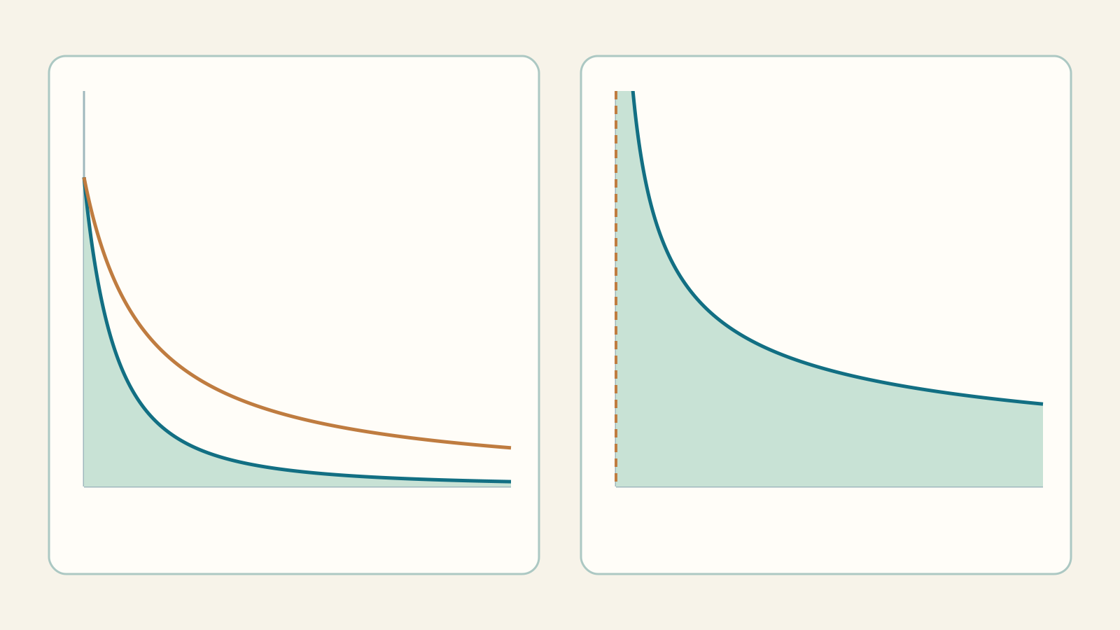
The lab has ten guided cases. The slider moves R from 1 to a million or ε from 1 to 10⁻⁶; multiple-cutoff cases start where all intervals are valid. Parameter α changes the ratio of left to right cutoff. Play advances one level per second.
The first plot shows the included region in a finite viewing window, with heights clipped if necessary. The second compares the total and, where needed, separate contributions. Values and tails come from the guided formulas, not quadrature of the drawing. Classification is theoretical; this is not a solver for arbitrary functions. Numbers are rounded.
Exercises: try before revealing
1. Find ∫1∞dx/x² and its remainder after R=1000.
Show the explained answer
I(R)=1−1/R, so the integral is 1. At R=1000 the truncated value is 0.999 and the omitted part is 0.001.
2. Which cutoff suffices for ∫01dx/√x with error at most 0.01?
Show the explained answer
The integral is 2 and the omitted part is 2√ε. We need ε≤(0.01/2)²=0.000025. The lab uses discrete levels and finds the first available cutoff meeting the bound.
3. Does unbounded −ln x near zero prevent a finite integral?
Show the explained answer
No: ∫ε1−ln x dx=1−ε+ε ln ε→1. An unbounded integrand need not give a divergent integral.
4. What is ∫−∞∞dx/(1+x²)? Must truncations be symmetric?
Show the explained answer
It is π: each tail converges separately to π/2. On [−L,R] the truncated value is arctan L+arctan R, tending to π regardless of growth rates.
5. For 1/x on [−1,1], what happens with cutoffs 2ε and ε?
Show the explained answer
The truncated total is ln 2, versus 0 for equal cutoffs. The ordinary integral does not converge: left −∞, right +∞. The symmetric principal value remains 0 and differs from the asymmetric-path limit.
6. Does symmetry make ∫−11dx/x² finite?
Show the explained answer
No: each side diverges to +∞. Equal cutoffs give 2/ε−2→+∞, so even the principal value is not finite.
7. How do we handle 1/√[x(1−x)] on (0,1)?
Show the explained answer
Separate the endpoints, for example at 1/2. Antiderivative 2 arcsin√x gives π/2 for each half: total π without equal cutoffs.
8. Do we need an antiderivative to prove convergence of ∫1∞dx/(1+x³)?
Show the explained answer
No: 0<1/(1+x³)≤1/x³ and ∫1∞dx/x³=1/2 is finite. Comparison proves convergence, not equality to 1/2.
Definite integrals and rotations · Series