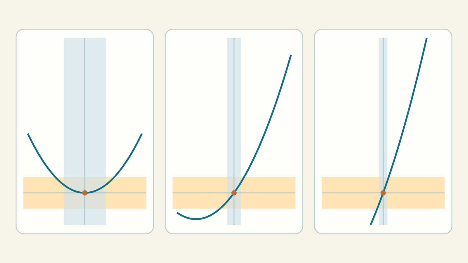
How close must two inputs be for their outputs to be close? Continuity answers around each individual point; uniform continuity asks for one input precision that works everywhere in the domain. This turns a local guarantee into a global one. We start with concrete examples, read quantifiers carefully and prove why compactness makes this possible. Limits, continuity and sequences are prerequisites; derivatives help but are not essential.
Lab: one δ for one point or for all? · Learning-path index
1. A precision requirement, not a matter of appearance
Suppose the allowed vertical error is less than ε=0.1. Choose a horizontal error δ so inputs less than δ apart give outputs less than ε apart. For f(x)=x², a small change near zero has little effect; near 100 the same input error can be greatly amplified. A curve without jumps does not by itself guarantee uniform precision.
|(100+0.001)²−100²|=0.200001
|(0+0.001)²−0²|=0.000001
The property always concerns a function together with its domain. Saying only “x² is uniformly continuous” is incomplete: yes on [−3,3], no on ℝ.
2. The two definitions and order of choices
Let f:D→ℝ. Continuity at every point means choosing center x₀, then tolerance ε, then a δ which may depend on both. For uniform continuity choose ε and then a single δ before knowing which x,y in the domain will be compared.
∀x₀∈D ∀ε>0 ∃δ=δ(ε,x₀)>0 ∀x∈D:
|x−x₀|<δ ⇒ |f(x)−f(x₀)|<ε

∀ε>0 ∃δ=δ(ε)>0 ∀x,y∈D:
|x−y|<δ ⇒ |f(x)−f(y)|<ε
“The same δ” does not mean one δ for every ε: reducing ε may require reducing δ. It means that after fixing ε, δ does not depend on the center. It may depend on the function and domain. All compared points must belong to D, including at interval endpoints. Uniform continuity implies continuity by setting y=x₀, but the converse fails in general.
3. Computing a local δ for x²
Fix x₀∈ℝ. Factor the difference of squares. If |x−x₀|<1, then |x+x₀|≤|x−x₀|+2|x₀|<1+2|x₀|. The following choice therefore suffices:
δ=min(1, ε/(2|x₀|+1))
|x²−x₀²|=|x−x₀||x+x₀|<δ(2|x₀|+1)≤ε
ε=0.1: x₀=0 ⇒ δ=0.1; x₀=100 ⇒ δ=0.1/201
We have proved continuity at every point. This choice is sufficient, not necessarily maximal. Seeing it shrink as the center grows does not alone prove no other uniform choice could exist. To disprove uniformity we will construct pairs defeating every δ.
4. The same function on [−M,M]
M>0; x,y∈[−M,M]
|x²−y²|=|x−y||x+y|≤2M|x−y|
δ=ε/(2M) ⇒ |x−y|<δ ⇒ |x²−y²|<ε
Now 2M bounds all locations at once: δ depends on ε and M, not x or y. On [−3,3], with ε=0.1, δ=1/60 suffices. This does not mean every pair farther apart must fail: the definition guarantees smaller distances, rather than giving a necessary condition for each individual pair.
For M=0 the domain is the singleton {0}: any δ>0 works because the same point is always compared. Do not divide by 2M in that case.
5. The Heine–Cantor theorem
If K⊂ℝ is compact and f:K→ℝ is continuous, then f is uniformly continuous on K. In ℝ, compact means closed and bounded. In particular, every continuous function on a closed bounded interval [a,b] is uniformly continuous. The result also applies to compact sets that are not intervals.
∀ε>0 ∃δ>0 ∀x,y∈K: |x−y|<δ ⇒ |f(x)−f(y)|<ε
The theorem guarantees existence of δ for each ε; it does not automatically supply an optimal formula. Differentiability is not required. Compactness is not claimed to be necessary: sin x on ℝ will disprove necessity, not the theorem itself.
Check both assumptions: a closed but unbounded domain may not suffice; a bounded but nonclosed domain may not suffice; continuity cannot be omitted even on [a,b].
6. Proof step by step using sequences
Assume for contradiction that f is not uniformly continuous. Negating the definition gives one fixed tolerance ε₀>0 violated for every positive δ, using a suitable pair each time. Take δ=1/n.
∃ε₀>0 ∀n≥1 ∃xₙ,yₙ∈K:
|xₙ−yₙ|<1/n; |f(xₙ)−f(yₙ)|≥ε₀
By compactness, xₙ has a subsequence xₙₖ converging to a point a belonging to K. This membership is crucial: f is continuous at a. Compare the matching subsequence yₙₖ:
|yₙₖ−a|≤|yₙₖ−xₙₖ|+|xₙₖ−a|<1/nₖ+|xₙₖ−a|→0
xₙₖ→a; yₙₖ→a
f(xₙₖ)→f(a); f(yₙₖ)→f(a)
|f(xₙₖ)−f(yₙₖ)|≤|f(xₙₖ)−f(a)|+|f(yₙₖ)−f(a)|→0
But the last difference was always at least ε₀, a contradiction. Thus f is uniformly continuous. The assumptions have distinct roles: compactness produces a limit point inside the domain, and continuity brings the images together.
7. Why x² is not uniformly continuous on ℝ
xₙ=n; yₙ=n+1/n
|yₙ−xₙ|=1/n→0
|yₙ²−xₙ²|=2+1/n²≥2
Inputs become arbitrarily close, but outputs do not. Fix ε₀=1: for every δ>0 choose an integer n>1/δ. Input distance is then less than δ while image distance exceeds ε₀. This negates the definition, rather than merely observing increasing slope.
There is no contradiction with Heine–Cantor: ℝ is closed but unbounded, hence noncompact. The same example works on [0,+∞).
8. Approaching an excluded endpoint
f(x)=1/x; D=(0,1]
xₙ=1/n; yₙ=1/(n+1)
|xₙ−yₙ|=1/[n(n+1)]→0
|f(xₙ)−f(yₙ)|=1
With ε₀=1/2 these pairs prove nonuniformity. f is continuous at every domain point, but zero is excluded: (0,1] is bounded and not closed. Both sequences converge precisely where continuity cannot be invoked.
f(x)=sin(1/x); D=(0,1]
xₙ=1/(2πn+π/2); yₙ=1/(2πn+3π/2), n≥1
xₙ,yₙ→0; |xₙ−yₙ|→0
f(xₙ)=1; f(yₙ)=−1
Here even the function is bounded between −1 and 1, yet the pair’s image gap is always 2. Continuity and boundedness on a bounded domain are not enough. Nor must a uniformly continuous function have bounded image: f(x)=x on ℝ is an immediate example.
9. Noncompact does not mean nonuniform
|sin x−sin y|≤|x−y|, x,y∈ℝ ⇒ δ=ε
|1/x−1/y|=|x−y|/(xy)≤|x−y|, x,y≥1 ⇒ δ=ε
The first inequality follows from the mean value theorem and |cos t|≤1. The second uses xy≥1. Thus sin x on ℝ and 1/x on [1,+∞) are uniformly continuous despite noncompact domains. The same expression 1/x gives different answers on different domains.
x≥y≥0; d=√x−√y≥0
x−y=d(√x+√y)≥d²
|√x−√y|≤√|x−y| ⇒ δ=ε²
√x on [0,+∞) is also uniformly continuous. Its derivative 1/(2√x), for x>0, is unbounded near zero, yet the inequality controls every pair. It is not Lipschitz near zero: |√h−0|/|h−0|=1/√h has no upper bound as h→0⁺.
10. Lipschitz bounds, derivatives and operations
A function is Lipschitz on D if some L≥0 satisfies |f(x)−f(y)|≤L|x−y| for all x,y∈D. For L>0 choose δ=ε/L; if L=0 the function is constant and any δ>0 works. Lipschitz continuity is therefore sufficient, not necessary, for uniform continuity.
Lipschitz ⇒ uniformly continuous ⇒ continuous
On an interval I, a continuous function differentiable in the interior with |f′|≤L is Lipschitz by the mean value theorem. The interval condition matters: the segment between points must lie in the domain. An unbounded derivative does not imply the contrary, as √x shows. A modulus of continuity ω(h) bounds |f(x)−f(y)| whenever |x−y|≤h and tends to zero as h→0; here ω(h)=Lh or √h.
Sums and compositions of uniformly continuous functions with compatible domains remain uniformly continuous. For composition, first choose the input tolerance required by the outer function, then δ for the inner one. Products need not: f(x)=g(x)=x are uniformly continuous on ℝ but fg=x² is not. Products do remain uniformly continuous if both functions are also bounded, using the following bound and splitting tolerance between its terms.
|f(x)g(x)−f(y)g(y)|
≤|f(x)||g(x)−g(y)|+|g(y)||f(x)−f(y)|
11. Why it matters: sequences, endpoints and sampling
A uniformly continuous function maps Cauchy sequences in its domain to Cauchy image sequences. Given ε, use the same δ for all sufficiently late pairs. This is not a characterization on every domain: x² on ℝ also maps Cauchy sequences to Cauchy sequences, yet is not uniformly continuous.
On a bounded interval (a,b), a real-valued f is uniformly continuous exactly when it extends continuously to [a,b]. For the less immediate direction, a sequence tending to a is Cauchy, so its images have a finite limit; interleaving two sequences shows the limit is independent of the choice. The same holds at b. Assign these endpoint values to obtain the continuous extension. Conversely apply Heine–Cantor to the extension and restrict to (a,b).
Finally, for continuous f on [a,b], a grid with every cell shorter than δ gives oscillation less than ε in each cell. Approximating f by one chosen value per cell gives integral error at most ε(b−a). This is a concrete reason uniform continuity matters numerically. Merely observing a finite grid without an analytical bound does not give that guarantee.
12. The lab: what to observe and what to prove
Choose one of seven cases and fix ε. In local mode, moving the center recalculates a sufficient δ for that center. In uniform mode, when the property holds, the same δ is kept as the center moves: the formula justifies every domain point, not only the animation’s twenty-one centers. The comparison table shows sufficient, not maximal, choices.
For the three nonuniform cases, propose δ: the program constructs x₀,x₁ with |x₁−x₀|<δ but image gap at least ε. Advancing reduces δ and builds another pair. The general proof is not the finite list of attempts, but the construction valid for every δ>0 described in the article.
Graph axes are relative: x−x₀ and f(x)−f(x₀). The blue band shows input proximity, the orange band allowed output error. Gray marks the center, red the second point. Automatic zoom is not the whole domain. For sin(1/x), sampled plotting may miss oscillations; the two extreme images are justified by the exact point formulas.
Exercises: try before revealing
1. May a uniform δ depend on ε?
Show the explained answer
Yes. Once ε is fixed, δ must work for every center in the domain. It need not be the same for different ε; it may depend on the function and domain.
2. Choose a uniform δ for x² on [−3,3] with ε=0.12.
Show the explained answer
|x²−y²|≤6|x−y|. δ=0.12/6=0.02 suffices: input distance <0.02 gives output error <0.12. This is a sufficient choice, not a claim of maximality.
3. For x², x₀=2 and ε=0.1, apply the local formula.
Show the explained answer
δ=min(1,0.1/(2·2+1))=0.02. Within δ of the center, |x+x₀|<5, hence |x²−x₀²|<5δ=0.1. The factor 5 concerns this center.
4. Why do xₙ=n and yₙ=n+1/n disprove uniform continuity of x²?
Show the explained answer
Distance 1/n tends to zero but the squares differ by 2+1/n². With ε₀=1, every δ is defeated by n>1/δ. xₙ need not converge: the domain is noncompact.
5. Compare 1/x on (0,1] and on [1,+∞).
Show the explained answer
On the first domain it is not uniform: 1/n and 1/(n+1) approach each other while images differ by 1. On the second |1/x−1/y|≤|x−y|, so δ=ε suffices. The expression alone is not enough.
6. Does an unbounded derivative rule out uniform continuity?
Show the explained answer
No. For √x on [0,+∞), |√x−√y|≤√|x−y|. With ε=0.1 choose δ=0.01. The derivative is unbounded near zero; the function remains uniform, though not Lipschitz near zero.
7. Does a noncompact domain prevent uniform continuity?
Show the explained answer
No: f(x)=x and f(x)=sin x on ℝ are uniformly continuous with δ=ε. Heine–Cantor gives a sufficient, not necessary, assumption. x on (0,1) is also uniform and extends continuously to its endpoints.
8. Continuous and bounded on a bounded set: enough?
Show the explained answer
No: sin(1/x) on (0,1] is continuous and bounded. Pairs xₙ=1/(2πn+π/2), yₙ=1/(2πn+3π/2) have distance tending to zero and images 1,−1. There is no limit at the excluded endpoint zero.
9. Does a step function on [−1,1] satisfy Heine–Cantor?
Show the explained answer
For f(x)=0 if x<0 and 1 if x≥0, the domain is compact but f is discontinuous at zero. With xₙ=−1/n and yₙ=0, images differ by 1. The continuity assumption is missing.
10. Prove uniform continuity of e^(−x) on [0,+∞).
Show the explained answer
|f′(x)|=e^(−x)≤1. The mean value theorem gives |f(x)−f(y)|≤|x−y|, so δ=ε suffices. The domain is an interval; compactness is not needed for this proof.
11. Is a product of uniformly continuous functions always uniform?
Show the explained answer
No: f=g=x on ℝ are uniformly continuous but fg=x² is not. If both are bounded too, the inequality in section 10 does give uniform continuity of the product.
12. For x² on [−3,3], ε=0.06, choose a grid with h<δ.
Show the explained answer
δ=ε/6=0.01. For N equal cells h=6/N: choose N=601 so h<0.01. Each cell’s oscillation is <0.06 and integral approximation error ≤0.06·6=0.36. This is sufficient, not an optimal grid.
Before: continuity and theorems · Learning-path index