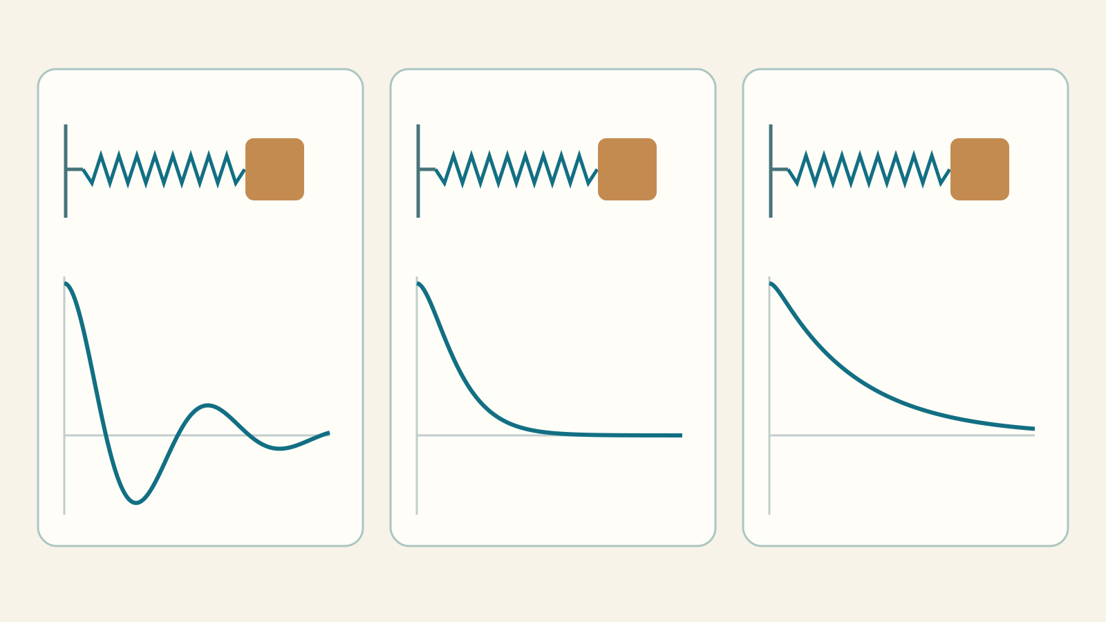
In the foundations we learned to describe change with a derivative. Now velocity itself changes: a spring accelerates a mass and resistance slows it down. We open the second block by building the model, deriving formulas and interpreting graphs. A memorised table is not enough: each solution must satisfy the equation and both initial conditions.
Lab: oscillations and second order · Learning-path index
1. Why a second derivative appears
Let x(t) be displacement from equilibrium, not absolute position. Its derivative x′(t) is velocity; the derivative of velocity x″(t) is acceleration. Second order means that x″ is the highest derivative present, not that the unknown is squared.
a₂(t)x″ + a₁(t)x′ + a₀(t)x = f(t), a₂(t) ≠ 0
The unknown is a function. The equation is linear when x, x′ and x″ occur only to the first power and do not multiply one another. x″+x=0 is linear; x″+x³=0 and x″+(x′)²=0 are not. We mainly develop constant-coefficient linear equations; general equations need other tools.
2. Two initial conditions: position and velocity
A snapshot does not reveal whether a body is stationary or passing rapidly. Predicting motion requires position and velocity at the same instant. Integrating x″=0 twice gives x′=C₂ and x=C₁+C₂t. The condition x(0)=2 fixes C₁=2 but leaves any velocity possible. Adding x′(0)=−3 selects one function.
x(0)=x₀, x′(0)=v₀; x″=0, x₀=2, v₀=−3 ⇒ x(t)=2−3t
If the coefficients and f are continuous on an interval and a₂ never vanishes, the linear initial-value problem has a unique solution on that interval. This is not a claim about every nonlinear equation. Conditions at different times, such as x(0)=0 and x(π)=0, form a boundary-value problem and may give no solution or many.
3. From an exponential to an algebraic equation
Start with the homogeneous equation: zero forcing and constant coefficients. An exponential is useful because its derivatives remain multiples of itself. Put x=eʳᵗ, so x′=reʳᵗ and x″=r²eʳᵗ. Substitute, factor and divide by eʳᵗ, which is never zero.
a₂x″+a₁x′+a₀x=0 ⇒ eʳᵗ(a₂r²+a₁r+a₀)=0 ⇒ P(r)=a₂r²+a₁r+a₀=0
We have turned the search for functions into a quadratic equation. Its roots are not values of x: they are the rates r in the exponentials. This characteristic equation works in this form because coefficients are constant. For t²x″+tx′−x=0, treating t as a constant and using the same recipe is not valid.
4. The three general-solution forms
Δ=a₁²−4a₂a₀
For Δ>0 there are two distinct real roots. The exponentials are independent and any linear combination solves the homogeneous equation. Choosing only one root would lose one of the two constants needed for initial conditions.
Δ>0: x=C₁e^(r₁t)+C₂e^(r₂t)
For Δ=0, repeating an exponential does not give two independent solutions: C₁eʳᵗ+C₂eʳᵗ is only (C₁+C₂)eʳᵗ. Substituting x=eʳᵗu gives a₂u″=0 because P(r)=0 and P′(r)=2a₂r+a₁=0. Thus u=C₁+C₂t: a factor t appears.
Δ=0: x=(C₁+C₂t)eʳᵗ
For Δ<0, roots are α±iβ with β>0. Real and imaginary parts of e⁽ᵅ⁺ⁱᵝ⁾ᵗ give two independent real functions, eᵅᵗcos(βt) and eᵅᵗsin(βt). The body does not need a complex displacement. The exponential controls amplitude; sine and cosine produce oscillation.
Δ<0: x=eᵅᵗ[C₁cos(βt)+C₂sin(βt)]
5. Three complete problems and their constants
First problem: solve x″+3x′+2x=0 with x(0)=0 and x′(0)=1. The characteristic polynomial factors as (r+1)(r+2)=0, so r₁=−1 and r₂=−2. Write both the general solution and its derivative before applying the data.
x=C₁e^(−t)+C₂e^(−2t);  x′=−C₁e^(−t)−2C₂e^(−2t)
C₁+C₂=0;  −C₁−2C₂=1  ⇒  C₁=1, C₂=−1
x=e^(−t)−e^(−2t)
Check: x″=e^(−t)−4e^(−2t). In the equation, coefficients of e^(−t) add to 1−3+2=0 and those of e^(−2t) to −4+6−2=0. Also x(0)=0 and x′(0)=−1+2=1. It leaves equilibrium with positive velocity, moves away and returns: a nonoscillatory motion need not be monotone.
Second problem: x″+4x′+4x=0, x(0)=1, x′(0)=0. Root −2 is repeated. In differentiating the product, retain the derivative of C₁+C₂t.
x=(C₁+C₂t)e^(−2t);  x′=[C₂−2(C₁+C₂t)]e^(−2t)
C₁=1;  C₂−2C₁=0  ⇒  C₂=2
x=(1+2t)e^(−2t);  x′=−4te^(−2t);  x″=(8t−4)e^(−2t)
Substitution gives (8t−4)−16t+4+8t=0. For t>0 velocity is negative, while x stays positive and tends to zero. This particular initial-value problem returns monotonically without crossing equilibrium.
Third problem: x″+2x′+5x=0, x(0)=1, x′(0)=0. Roots are −1±2i. At zero, cosine is 1 and sine is 0. Initial velocity includes both the exponential derivative and the sine derivative.
x=e^(−t)[C₁cos(2t)+C₂sin(2t)]
x(0)=C₁=1;  x′(0)=−C₁+2C₂=0  ⇒  C₂=1/2
x=e^(−t)[cos(2t)+(1/2)sin(2t)]
This motion oscillates with decreasing amplitude. The trigonometric factor has period π, but the full function is not periodic: after π its exponential amplitude has changed. Verify the equation by differentiating twice or by using the two independent solutions already obtained from the characteristic roots.
6. Building a mass–spring model
Choose a horizontal axis and measure x from equilibrium. An ideal spring exerts −kx, with the negative sign pointing towards zero. A viscous damper exerts −cx′, opposing velocity. An external agent applies F(t). Newton’s second law equates mass times acceleration to the sum of forces.
mx″=−cx′−kx+F(t)  ⇒  mx″+cx′+kx=F(t)
m>0, k>0, c≥0
With t in seconds and x in metres, m is in kg, k in N/m, c in N·s/m and F in newtons. Each term has force dimensions. For a vertical spring, gravity shifts equilibrium; measuring x from that equilibrium cancels the constant weight term. Do not add it again without changing the reference.
For m=1, k=4, c=0 and F=0, the characteristic equation is r²+4=0. Releasing from x₀=1 with v₀=0 gives x=cos(2t), v=−2sin(2t). Natural angular frequency is 2 rad/s, period π seconds and frequency 1/π hertz: frequency and angular frequency differ.
7. Undamped, underdamped, critical and overdamped
Set F=0 and divide by m. The following quantities separate system properties from initial conditions. Critical damping follows by setting the discriminant of mr²+cr+k=0 to zero.
ω₀=√(k/m),  γ=c/(2m),  c_crit=2√(mk)
r=−γ±√(γ²−ω₀²)
For c=0 the ideal system keeps oscillating. If 0<c<c_crit, roots are complex: damped oscillation has ω_d=√(ω₀²−γ²), below ω₀. One trigonometric cycle lasts 2π/ω_d. The exponential e^(−γt) reduces the envelope; it does not shorten the period.
0≤c<c_crit: x=e^(−γt)[x₀cos(ω_dt)+(v₀+γx₀)sin(ω_dt)/ω_d]
c=c_crit: x=e^(−γt)[x₀+(v₀+γx₀)t]
At critical damping the root is repeated. For c>c_crit, both roots are real and negative and free response is a sum of decaying exponentials. Very large c can slow the return as one root approaches zero. Nonoscillatory does not mean never crossing zero: some initial velocities cause a crossing even in critical or overdamped cases.
c>c_crit: C₁=(v₀−r₂x₀)/(r₁−r₂), C₂=(r₁x₀−v₀)/(r₁−r₂)
x=C₁e^(r₁t)+C₂e^(r₂t)
Concrete comparison: fix m=k=1, x₀=1 and v₀=0. Values c=0, 0.5, 2 and 4 give harmonic, underdamped, critical and overdamped motion. This comparison is meaningful because mass, stiffness and initial data stay fixed.
8. Energy checks whether a solution is plausible
Mechanical energy is kinetic plus elastic energy. Differentiate, factor x′ and substitute the equation of motion. No explicit formula for x(t) is needed.
E=(1/2)m(x′)²+(1/2)kx²
E′=mx′x″+kxx′=x′(mx″+kx)=F(t)x′−c(x′)²
With no external force, c=0 keeps energy constant and c>0 makes it nonincreasing. At an instant with x′=0, E′ may be zero even when c>0; this does not remove damping. With forcing, F(t)x′ is input power and can balance dissipation. An algorithm inventing energy growth in free dissipative motion needs numerical checking.
9. External forcing: homogeneous plus particular
For nonzero F, solving the characteristic equation is not enough. If x_p solves the full equation and x_h solves the associated homogeneous equation, linearity gives L[x_h+x_p]=0+F. Conversely, the difference of two full solutions is homogeneous. This explains the structure of every solution.
x=x_h+x_p
Example: x″+3x′+2x=2, x(0)=0, x′(0)=0. Try a constant particular solution A: its derivatives vanish and 2A=2, so A=1. Apply initial conditions to the full sum, not just x_h.
x=C₁e^(−t)+C₂e^(−2t)+1
C₁+C₂=−1;  −C₁−2C₂=0  ⇒  C₁=−2, C₂=1
x=1−2e^(−t)+e^(−2t)=(1−e^(−t))²
The limit is 1, not zero: constant forcing shifted equilibrium. Undetermined coefficients use a trial form matching F: polynomial, exponential, sine and cosine. If the trial already belongs to the homogeneous solution space, multiply by t to the multiplicity of the corresponding root. More general forces need variation of parameters or numerical methods; the root table does not replace them.
10. Periodic forcing and resonance
For F(t)=F₀cos(Ωt), try x_p=Acos(Ωt)+Bsin(Ωt). Differentiating twice and collecting sine and cosine gives a linear system for A and B. Put D=k−mΩ² and Q=D²+(cΩ)². The system is invertible when Q>0.
DA+cΩB=F₀;  DB−cΩA=0
A=F₀D/Q;  B=F₀cΩ/Q
x_p=F₀[Dcos(Ωt)+cΩsin(Ωt)]/Q
For m=1, c=1, k=4, F₀=1 and Ω=2, D=0 and Q=4, giving x_p=(1/2)sin(2t). This is particular, not automatically the zero-initial-data solution: its initial velocity is 1, so a homogeneous transient must correct it. With c>0 the free transient decays, leaving bounded periodic response.
R(Ω)=F₀/√[(k−mΩ²)²+(cΩ)²]
If c=0 and Ω=ω₀, Q vanishes: the formula is undefined, not a finite number turning into infinity. Instead solve that equation. For zero initial data a resonant particular solution is proportional to t sin(ω₀t).
c=0, Ω=ω₀, x₀=v₀=0:  x(t)=F₀t sin(ω₀t)/(2mω₀)
x″+x=cos(t), x(0)=x′(0)=0  ⇒  x=(t/2)sin(t)
Check the last example: x′=(1/2)sin(t)+(t/2)cos(t), x″=cos(t)−(t/2)sin(t), hence x″+x=cos(t). Its envelope grows linearly in the ideal model. Real friction, nonlinearities and structural limits prevent unrestricted extrapolation to any amplitude.
Distinguish natural ω₀, damped-transient ω_d and imposed driving Ω. For c>0 and c²<2mk, steady displacement amplitude peaks at Ω_r=√(k/m−c²/(2m²)), not exactly ω₀. With stronger damping this amplitude has no positive-frequency peak. Unbounded ideal resonance concerns the undamped case.
11. From model to lab: keeping approximations explicit
In the lab choose a case, change m, c, k, x₀ and v₀ and apply. The plot shows displacement over time; the animated spring shows the same value at each instant. Step manually or play: one second between frames need not mean one physical second. Drawing scale adapts to the observed interval and is illustrative.
Free motion and undamped forcing use analytical formulas, still evaluated in floating point. With both forcing and damping, the lab explicitly uses fourth-order Runge–Kutta with small internal steps: not a symbolic solution or a certified error guarantee. The table compares position, velocity and energy.
v=x′; x′=v, v′=[F₀cos(Ωt)−cv−kx]/m
Rewriting as two first-order equations explains the numerical calculation and prepares, but does not replace, the future systems chapter. Try varying only c across regimes; changing initial velocity; comparing constant forcing (Ω=0) with periodic forcing; then adding damping to ideal resonance. The lab restricts m,k to positive values and c to nonnegative values; it does not cover every second-order equation.
12. A workflow that keeps every step
First identify order, linearity and coefficients; distinguish initial and boundary data. Use a characteristic equation for the homogeneous part only with constant coefficients. Write two independent solutions, add a particular solution when needed, differentiate and use both initial conditions to find constants. Finally check equation, data, units and time behaviour.
Common errors include missing t for a repeated root, imposing data only on the homogeneous part, calling a decaying-envelope curve periodic, dividing by Q=0 at resonance or treating a numerical plot as a proof. Connections to the foundations are concrete: derivatives for modelling and checks, limits for stability, trigonometry for oscillations and integrals for energy and work.
Exercises: try before revealing
1. Solve x″=0 with x(0)=3 and x′(0)=−2.
Show the explained answer
Integrate: x′=C₂ and x=C₁+C₂t. The data give C₁=3 and C₂=−2, hence x=3−2t. Its second derivative is zero and both conditions hold.
2. Solve x″+3x′+2x=0, x(0)=1, x′(0)=0.
Show the explained answer
Roots are −1 and −2. For x=C₁e^(−t)+C₂e^(−2t), the data give C₁+C₂=1 and −C₁−2C₂=0, hence C₁=2 and C₂=−1. Thus x=2e^(−t)−e^(−2t).
3. Solve x″+2x′+x=0, x(0)=2, x′(0)=−1.
Show the explained answer
Root −1 is repeated: x=(C₁+C₂t)e^(−t). C₁=2 and x′(0)=C₂−C₁=−1 give C₂=1. Thus x=(2+t)e^(−t), not 2e^(−t), whose initial velocity would be −2.
4. Solve x″+9x=0, x(0)=0, x′(0)=6; find period and energy for m=1.
Show the explained answer
x=C₁cos(3t)+C₂sin(3t). C₁=0 and 3C₂=6 give x=2sin(3t), v=6cos(3t). Period is 2π/3 and E=(1/2)36cos²(3t)+(1/2)9·4sin²(3t)=18.
5. For m=4 and k=9, find critical c and solve for x₀=1, v₀=0.
Show the explained answer
c_crit=2√(4·9)=12 and γ=12/8=3/2. Critical response is x=[1+(3/2)t]e^(−3t/2). Do not use c_crit=2k: mass belongs inside the square root.
6. Solve x″+4x′+13x=0 with x(0)=0 and x′(0)=3.
Show the explained answer
Roots are −2±3i. x=e^(−2t)[C₁cos(3t)+C₂sin(3t)]. Initial data give C₁=0 and 3C₂=3: x=e^(−2t)sin(3t). Its trigonometric factor has period 2π/3; the full solution is not periodic.
7. For 2x″+3x′+4x=8, what equilibrium and limit do you expect?
Show the explained answer
A constant equilibrium satisfies 4x_eq=8, so x_eq=2. Homogeneous roots have real part −3/4<0; the transient decays and every finite-initial-data solution tends to 2. Forced equilibrium is not necessarily zero.
8. Can critical motion cross equilibrium? Try x″+2x′+x=0, x₀=1, v₀=−3.
Show the explained answer
x=e^(−t)[1+(−3+1)t]=(1−2t)e^(−t). The exponential stays positive, so x crosses zero at t=1/2 and becomes negative. One crossing is not repeated oscillation. Critical damping alone does not determine the whole motion without initial data.
9. Find a particular solution of x″−x=eᵗ. Why does Aeᵗ fail?
Show the explained answer
eᵗ is already homogeneous: (Aeᵗ)″−Aeᵗ=0. Try x_p=Ateᵗ. Then x_p′=A(1+t)eᵗ and x_p″=A(2+t)eᵗ, so x_p″−x_p=2Aeᵗ. Hence A=1/2 and x=C₁eᵗ+C₂e^(−t)+(t/2)eᵗ.
10. Solve x″+4x=cos(2t), x₀=v₀=0 and evaluate x(π/4).
Show the explained answer
Ideal resonance has m=1, ω₀=Ω=2, F₀=1. Thus x=(t/4)sin(2t), already satisfying zero initial data. At t=π/4, sin(π/2)=1 and x=π/16. Do not divide by k−mΩ²=0.
11. For m=1, c=1, k=4, F₀=1 find steady amplitude at Ω=2 and the peak angular frequency.
Show the explained answer
R(2)=1/√[(4−4)²+2²]=1/2. A peak exists since c²=1<2mk=8 and occurs at Ω_r=√(4−1/2)=√(7/2), not 2. Amplitude is finite, unlike unbounded undamped resonance.
12. In free motion with m=k=1, c=1/2, x=2, v=3, find E and E′.
Show the explained answer
E=(1/2)·3²+(1/2)·2²=13/2. Since F=0, E′=−cv²=−9/2: energy is decreasing at that instant. Reconstructing the whole motion also requires a reference time and initial conditions.
Before: first-order differential equations · Learning-path index