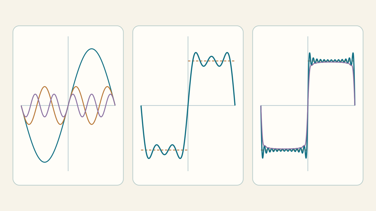
A periodic signal may look square, triangular or irregular: its Fourier series studies it through simple oscillations. But adding sines and cosines is not enough: we must choose coefficients, identify the sum’s limit and specify the error being measured. We start with period and orthogonality, work examples and reach Gibbs, Fejér means and spectra. Integrals, trigonometry and sequences and series of functions are prerequisites.
Lab: building a Fourier series · Learning-path index
1. Period, frequency and harmonics
f(t+T)=f(t); T>0
ν₀=1/T; ω₀=2π/T
cos(nω₀t), sin(nω₀t); n=1,2,…
The fundamental completes one oscillation in T; harmonic n completes n. If t is seconds, n/T is frequency in hertz and nω₀ angular frequency in radians per second. N is the highest included harmonic, not the count of nonzero terms: harmonics 1,3,5 require N=5.
Taylor uses polynomials near a point; Fourier uses trigonometric functions over an entire period. Assigning a function on an interval and extending it periodically makes endpoint joins part of the problem: they may introduce jumps even if the interior segment is smooth.
2. Orthogonality: where coefficients come from
On [−π,π], integer-frequency sines and cosines are orthogonal: different modes have zero product integral. Use product-to-sum identities, for example 2cos(nθ)cos(mθ)=cos((n−m)θ)+cos((n+m)θ). When n=m a constant term remains.
∫₋π^πcos(nθ)cos(mθ)dθ=πδₙₘ
∫₋π^πsin(nθ)sin(mθ)dθ=πδₙₘ
∫₋π^πsin(nθ)cos(mθ)dθ=0; n,m≥1
∫₋π^π1dθ=2π
δₙₘ is 1 if n=m and 0 otherwise. For our square-integrable examples, choose a degree-N trigonometric polynomial minimizing integrated squared error; orthogonality separates the coefficients. We need not assume an infinite series identity before proving it: define coefficients first, then study convergence.
S_N(t)=a₀/2+Σₙ₌₁ᴺ[aₙcos(nω₀t)+bₙsin(nω₀t)]
aₙ=(2/T)∫₋T/2^T/2 f(t)cos(nω₀t)dt, n≥0
bₙ=(2/T)∫₋T/2^T/2 f(t)sin(nω₀t)dt, n≥1
a₀/2=(1/T)∫₋T/2^T/2 f(t)dt
For T=2L, factor 2/T becomes 1/L and nω₀ becomes nπ/L. The constant term is a₀/2 because the squared norm of 1 is twice that of each sine or cosine. Missing this factor incorrectly doubles the mean.
3. Symmetry, amplitude and phase
If f is even on a centered period, bₙ vanish because odd integrands integrate to zero. If f is odd, a₀ and all aₙ vanish. Symmetry halves the work, but check the function and period center before dropping terms.
aₙcos(nω₀t)+bₙsin(nω₀t)=Rₙcos(nω₀t−φₙ)
Rₙ=√(aₙ²+bₙ²); φₙ=atan2(bₙ,aₙ)
Spectral amplitude Rₙ is nonnegative while aₙ,bₙ may have either sign. If Rₙ=0 phase is undefined: the table shows a dash, not an arbitrary phase. The mean is separately a₀/2; its plotted amplitude is |a₀/2|, not |a₀|.
4. Square wave: complete calculation
On normalized period (−π,π), take g(θ)=−1 for θ<0 and +1 for θ>0, assigning midpoint 0 at jumps. Oddness gives a₀=aₙ=0. For sine coefficients integrate only the positive half:
bₙ=(2/π)∫₀^πsin(nθ)dθ
=(2/π)[−cos(nθ)/n]₀^π
=2[1−(−1)ⁿ]/(πn)
b₂ₖ=0; b₂ₖ₊₁=4/[π(2k+1)]
S_N(θ)=(4/π)Σₖ₌₀^⌊(N−1)/2⌋ sin((2k+1)θ)/(2k+1)
N=5 includes three nonzero harmonics; N=6 gives the same ordinary sum since coefficient 6 is zero. Fejér means can change between 5 and 6 because weights of existing harmonics also change.
5. Sawtooth: watch the periodic join
Take g(θ)=θ/π for −π<θ<π and repeat it. This is odd too, but sine coefficients alternate signs. Integrate by parts with u=θ and dv=sin(nθ)dθ:
bₙ=(2/π²)∫₀^πθsin(nθ)dθ
=(2/π²)[−θcos(nθ)/n+sin(nθ)/n²]₀^π
=2(−1)^(n+1)/(πn)
g(θ)∼(2/π)[sinθ−sin(2θ)/2+sin(3θ)/3−⋯]
Here ∼ denotes the associated Fourier series, not equality at every assigned point. At θ=π the left limit is +1 and the right limit −1, so the series converges to 0. A smooth linear segment can therefore create endpoint Gibbs behavior after periodic extension.
6. Corners without jumps and other lab signals
Triangle wave g(θ)=(2/π)arcsin(sinθ) is odd and continuous, including period joins. Integrating by parts on the two linear pieces of [0,π], split at π/2, gives alternating odd sine coefficients. For even |θ|/π, instead integrate θcos(nθ) on [0,π].
g(θ)=(2/π)arcsin(sinθ): a₀=aₙ=0; bₙ=8sin(nπ/2)/(π²n²)
g(θ)=|θ|/π: a₀=1; bₙ=0
aₙ=(2/π²)[θsin(nθ)/n+cos(nθ)/n²]₀^π
=2[(−1)ⁿ−1]/(π²n²)
Coefficients decay as 1/n²: their absolute sum converges, so the M-test gives uniform convergence. A corner is not a jump in value; the jump-specific Gibbs constant should not automatically be applied to it. Two further continuous examples are the periodic parabola and half-wave sine:
g(θ)=(θ/π)²: a₀=2/3; aₙ=4(−1)ⁿ/(π²n²); bₙ=0
g(θ)=max(0,sinθ): a₀=2/π; b₁=1/2
a₂ₖ=−2/[π(4k²−1)], k≥1; a₂ₖ₋₁=0; bₙ=0 (n>1)
For a centered unit-height pulse occupying fraction q of a period, symmetry gives cosines only. Integrating over [−πq,πq] gives mean q and the following coefficients; the lab assigns 1/2 at both jumps.
a₀=2q; aₙ=2sin(nπq)/(πn); bₙ=0
7. To which value does the series converge?
A convenient sufficient assumption is that the periodic extension is piecewise C¹, with finitely many pieces and finite one-sided limits of the function and derivatives at breakpoints. Ordinary partial sums then converge to the midpoint of the one-sided limits:
lim_N→∞ S_N(t)=[f(t⁻)+f(t⁺)]/2
At continuity points the midpoint is f(t). At a jump it may differ from the assigned point value. Altering finitely many values does not change coefficient integrals, so the series cannot recover arbitrary isolated values. At period endpoints compare both sides of the periodic extension, not only the plotted segment.
Every S_N is continuous, so it cannot converge uniformly over a period to a function with jumps. Our discontinuous examples may improve away from jumps without global uniformity. For continuous examples with absolutely summable coefficients, the M-test does guarantee uniformity. A close-looking plot does not replace these assumptions.
8. Gibbs: the peak narrows, not vanishes
For the square wave let M=⌊(N+1)/2⌋, the number of odd harmonics. Differentiate the finite sum and use the cosine-sum identity to locate the first maximum to the right of the jump. No infinite-series differentiation theorem is needed for a finite sum.
S_N′(θ)=(4/π)Σⱼ₌₀ᴹ⁻¹cos((2j+1)θ)
=(2/π)sin(2Mθ)/sinθ
θ*=π/(2M); t*=T/(4M)
lim_M→∞S_N(θ*)=(2/π)∫₀^π sin u/u du≈1.178979744
The last limit is a Riemann sum for the sine integral. High level is 1 and jump is 2: excess is about 0.17898, or 8.949% of the jump, not of high amplitude 1. For a jump J, limiting overshoot is about 0.08949J. Small-N percentages may differ; the lab evaluates the actual finite sum at t*.
The peak distance is of order 1/N, so the problematic region shrinks. This does not contradict pointwise convergence: t* moves with N instead of remaining fixed.
9. Fejér means: same coefficients, different weights
σ_N=(S₀+S₁+⋯+S_N)/(N+1)
=a₀/2+Σₙ₌₁ᴺ(1−n/(N+1))[aₙcos(nω₀t)+bₙsin(nω₀t)]
Harmonic n appears in S_n through S_N, exactly N+1−n times, giving its weight. The average is not over only nonzero modes and includes S₀=a₀/2. High frequencies are attenuated more than low ones.
F_N(u)=(1/(N+1))[sin((N+1)u/2)/sin(u/2)]²≥0; u∉2πℤ
F_N(2kπ)=N+1; k∈ℤ
(1/(2π))∫₋π^πF_N(u)du=1
σ_N(θ)=(1/(2π))∫₋π^πg(θ−u)F_N(u)du
On the normalized period, kernel F_N is nonnegative with total mass 1, making σ_N a weighted average of signal values and keeping it within their range. Fejér means converge uniformly for every continuous periodic function: uniform continuity controls nearby contributions, while kernel mass away from zero tends to zero.
At jumps of our signals, the midpoint limit remains; global uniform convergence to a discontinuous function is still impossible. Fejér removes overshoot beyond signal levels but broadens transitions: it does not reduce every error at the same N.
10. Parseval, RMS and best quadratic approximation
For square-integrable f, completeness of the trigonometric system in L² gives Parseval’s identity. We use the period average rather than total integral: its units are amplitude squared, independent of the chosen T.
(1/T)∫₋T/2^T/2 |f(t)|²dt=a₀²/4+(1/2)Σₙ₌₁∞(aₙ²+bₙ²)
RMS_N²=(1/T)∫₋T/2^T/2|f−S_N|²dt=(1/2)Σₙ>N(aₙ²+bₙ²)
Orthogonality also proves optimality: for any other trigonometric polynomial P_N of degree at most N, squared error equals that of S_N plus squared distance between S_N and P_N. The cross term vanishes. Thus S_N minimizes RMS, not necessarily maximum pointwise error.
RMS²(f−P_N)=RMS²(f−S_N)+RMS²(S_N−P_N)
RMS²(f−σ_N)=RMS²(f−S_N)
+(1/2)Σₙ₌₁ᴺ[n/(N+1)]²(aₙ²+bₙ²)
Normalized square-wave mean square is 1; sawtooth and triangle have mean square 1/3. Lab integrals and coefficients are analytical, not estimated from plots. Small RMS can coexist with Gibbs: narrow regions contribute little to an integral but still matter for uniform error.
11. Amplitude, mean level, period and complex form
f(t)=C+A g(2πt/T)
a₀(f)=2C+A a₀(g)
aₙ(f)=A aₙ(g); bₙ(f)=A bₙ(g), n≥1
In the lab, changing T stretches the signal while keeping normalized profile g fixed. Frequencies n/T change, not coefficient amplitudes. A scales variable components; C changes only the mean term. If g has mean μ, f has mean C+Aμ: C is not necessarily the total mean.
cₖ=(1/T)∫₋T/2^T/2 f(t)e^(−ikω₀t)dt
c₀=a₀/2; cₙ=(aₙ−ibₙ)/2; c₋ₙ=(aₙ+ibₙ)/2
S_N(t)=Σₖ₌₋ᴺᴺcₖe^(ikω₀t)
The complex form is the same representation using e^(iθ)=cosθ+i sinθ. For real f, c₋ₙ is the conjugate of cₙ, so paired complex terms give a real result. For n>0, real amplitude Rₙ=2|cₙ|, not |cₙ|.
12. Applications: heat, signals and sampling limits
For periodic heat flow in θ, harmonics evolve separately. Equation u_τ=κu_θθ with κ>0 and initial profile g(θ) attenuates mode n by e^(−κn²τ): finer structure decays faster. For τ>0 this factor strongly smooths the series; the mean stays unchanged.
u(θ,τ)=a₀/2+Σₙ₌₁∞e^(−κn²τ)[aₙcos(nθ)+bₙsin(nθ)]
For signals, the spectrum identifies contributing frequencies, amplitudes and phases. Fourier series concern periodic functions and discrete frequencies; the Fourier transform is a different tool, typically for nonperiodic signals and continuous frequencies. A DFT uses finitely many samples and does not automatically equal analytical coefficient integrals.
θⱼ=2πj/M ⇒ cos(Mθⱼ)=1, j=0,…,M−1
This demonstrates aliasing: a genuine order-M harmonic looks constant at sample nodes. A sampled plot can hide oscillations or suggest incorrect coefficients. The lab uses analytical coefficient formulas while explicitly treating plots as sampled illustrations.
13. A full example: period 4, amplitude 2, level 1
Let g be the normalized square wave and f(t)=1+2g(πt/2). T=4, ω₀=π/2 and mean 1. Levels are −1 and 3, a jump of 4. Three nonzero harmonics require N=5.
a₀=2; aₙ=0
bₙ=8/(πn) (n=1,3,5,…); b₂ₖ=0
S₅(t)=1+(8/π)[sin(πt/2)+sin(3πt/2)/3+sin(5πt/2)/5]
S₅(0)=1
S₅(1)=1+(8/π)(1−1/3+1/5)=1+104/(15π)≈3.207
At t=0 the sum gives midpoint 1 of the jump. At t=1 the target is 3 and the finite sum exceeds it, but this is not the first peak near the jump: M=3 gives t*=T/(4M)=1/3. An observed value is not automatically a graph maximum.
RMS₅²=4[1−(8/π²)(1+1/9+1/25)]
The final formula measures squared error averaged over the whole period. It does not bound every point error by RMS: near jumps that error may be much larger.
14. The lab and a study procedure
Choose one of eight signals and edit A,C,T,N; the pulse also allows q. The first plot compares f and S_N, with optional σ_N. Zoom follows a jump without changing the periodic domain. Slider h isolates one harmonic, with h=0 for the mean. The spectrum shows amplitudes; the table keeps signed coefficients and phases.
RMS errors come from Parseval. For absolutely summable coefficients we also show uniform-error upper bounds from coefficient tails: sufficient bounds, not necessarily exact maxima for each method. Jumping signals instead show an obstruction of at least half the jump: a continuous approximant must err on one side. The maximum over 401 window samples is explicitly sampled and may underestimate global error.
The last signal is already finite: g(θ)=0.1+0.6cosθ+0.3sin(2θ)−0.2cos(3θ). From N=3 ordinary sums are exact in the model, but Fejér still attenuates modes: smoothing is not minimization of every error. General procedure: choose period and extension, check symmetry, compute coefficients, state convergence type, then interpret plots and errors.
Exercises: try before revealing
1. A function has period T=4. What are the fundamental and third-harmonic frequencies?
Show the explained answer
ν₀=1/T=1/4; ω₀=2π/T=π/2. The third harmonic has frequency 3/T=3/4 and angular frequency 3π/2. Frequency and angular frequency are different quantities.
2. For f(t)=3, what are a₀ and the mean?
Show the explained answer
a₀=(2/T)·3T=6. The mean is a₀/2=3; all other coefficients vanish. The constant-term factor 1/2 is essential.
3. Which coefficients vanish for the odd square wave?
Show the explained answer
Oddness kills a₀ and all aₙ. Here bₙ=2[1−(−1)ⁿ]/(πn): even indices vanish, odd indices give 4/(πn). Oddness alone does not generally kill even-index bₙ.
4. Do N=5 and N=6 give the same square-wave approximation?
Show the explained answer
Yes for S_N: harmonic 6 is zero, leaving 1,3,5. Not for σ_N: weights change from 1−k/6 to 1−k/7 on existing modes. N is the highest index, not the number of nonzero terms.
5. The sawtooth equals θ/π on (−π,π). What is the series limit at π?
Show the explained answer
The periodic one-sided limits are 1 and −1, so the series converges to (1−1)/2=0. Changing only the assigned value at π does not change coefficient integrals.
6. Why does the series of |θ|/π converge uniformly?
Show the explained answer
Mean 1/2; bₙ=0 and aₙ=−4/(π²n²) for odd n, zero for even n. Terms are bounded by the summable sequence 4/(π²n²). The M-test gives uniform convergence to the continuous periodic extension.
7. A centered pulse occupies 40% of the period. Find its mean and first coefficient.
Show the explained answer
q=0.4. Mean q=0.4 and a₀=0.8. Symmetry gives bₙ=0; a₁=2sin(0.4π)/π≈0.60546. Height and relative duration are distinct.
8. What is the asymptotic Gibbs overshoot for a jump from −1 to 3?
Show the explained answer
Jump J=4. Overshoot tends to 0.089489872…·4≈0.3579595 above level 3, so the first peak tends to 3.3579595. The percentage refers to jump size, not high level. Finite-N values differ.
9. Which weights does Fejér use for N=3?
Show the explained answer
σ₃=(S₀+S₁+S₂+S₃)/4. Harmonic 1 occurs three times, 2 twice, 3 once: weights 3/4,1/2,1/4. The mean occurs in every sum and stays unchanged.
10. For f(θ)=2cos(3θ), find RMS error at N=2 and N=3.
Show the explained answer
Only a₃=2 is nonzero. S₂=0, so RMS²=(1/2)·2²=2 and RMS=√2. S₃=f, so RMS=0. The factor 1/2 is the period mean of cos².
11. Does Fejér smoothing always improve RMS error?
Show the explained answer
No. For g=0.1+0.6cosθ+0.3sin2θ−0.2cos3θ, S₃=g and RMS=0. σ₃ attenuates already exact coefficients; its RMS is √[(0.15²+0.15²+0.15²)/2]=√0.03375≈0.18371. Ordinary sums are the degree-constrained optimal quadratic projection.
12. For T=4,A=2,C=1,N=5, is the value at t=1 the first peak?
Show the explained answer
No. S₅(1)=1+104/(15π)≈3.207. There are M=3 odd harmonics; the first peak near the jump at 0 is at t*=T/(4M)=1/3. At t=0 the sum is midpoint 1.
Before: sequences and series of functions · Learning-path index