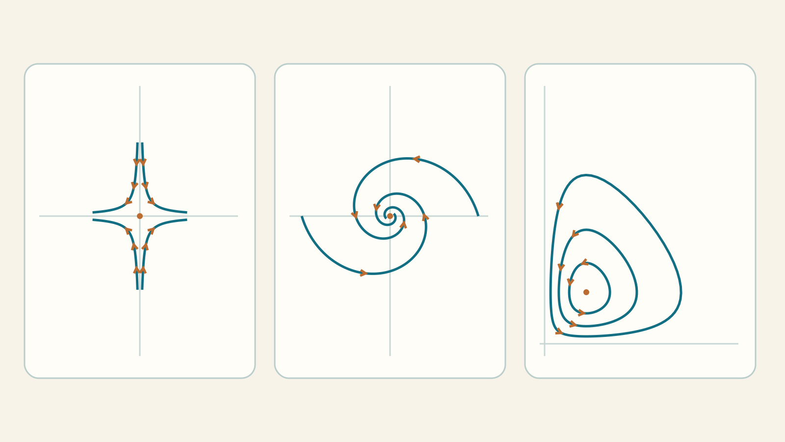
One population changes another; velocity changes position and position changes acceleration. When quantities interact, one equation is not enough. We learn to write the system, find equilibria and solutions, read plots and check computer calculations. Derivatives, exponentials and basic vectors are prerequisites; matrices and eigenvalues are introduced here.
Lab: systems, trajectories and equilibria · Learning-path index
1. State and initial-value problem
The state is the pair (x(t),y(t)), specifying both quantities at one instant. The unknowns are two functions, not two numbers. A first-order system prescribes both rates of change.
x′ = f(t,x,y)
y′ = g(t,x,y)
x(t₀)=x₀, y(t₀)=y₀
If f and g do not explicitly depend on t, the system is autonomous. With f,g continuous and locally Lipschitz in (x,y), initial data determine a unique local solution. Our polynomial fields satisfy this condition, but for a nonlinear system this alone does not guarantee a solution for all time.
2. Start with independent equations
x′=−x, y′=−2y; x(0)=2, y(0)=3
x(t)=2e^(−t), y(t)=3e^(−2t)
Each equation can be solved separately: x does not use y and vice versa. Differentiating recovers −x and −2y; setting t=0 recovers 2 and 3. Both coordinates approach zero, but y decays faster.
e^(−t)=x/2 ⇒ y=3(x/2)²=(3/4)x², x>0
In the (x,y) plane the trajectory is a parabola arc followed toward the origin. The time plots instead show two exponentials. These are different descriptions of the same motion: time is not an axis in the phase plane.
3. Arrows, nullclines and equilibria
For an autonomous system, at each (x,y) draw the vector (f(x,y),g(x,y)). It gives the oriented tangent to the motion. The lab normalizes arrows, retaining direction but not speed.
x′=0 ⇔ f(x,y)=0
y′=0 ⇔ g(x,y)=0
(f(x*,y*),g(x*,y*))=(0,0)
On the first nullcline the tangent is vertical if g≠0; on the second it is horizontal if f≠0. A nullcline is not generally a trajectory. At an intersection the state stays constant. With uniqueness, distinct orbits cannot cross at a nonstationary point; a closed orbit can, however, be traversed periodically.
4. Linear systems: matrices and eigenvalues step by step
x′=ax+by, y′=cx+dy
z=(x,y)ᵀ; M=[[a,b],[c,d]]; z′=Mz
The matrix is a coefficient table: its first row produces x′ and its second y′. Seek motion along a fixed direction v=(v₁,v₂): z(t)=e^(λt)v, v≠0. Differentiation and cancellation give Mv=λv: v is an eigenvector and λ its eigenvalue.
(a−λ)v₁+bv₂=0; cv₁+(d−λ)v₂=0
det(M−λI)=(a−λ)(d−λ)−bc=0
λ²−(a+d)λ+(ad−bc)=0
τ=a+d; D=ad−bc; Δ=τ²−4D
λ₁,₂=(τ±√Δ)/2
Zero determinant allows a nonzero v. With distinct real eigenvalues, the two eigenvectors are independent: z=C₁e^(λ₁t)v₁+C₂e^(λ₂t)v₂. Initial data determine C₁,C₂. Complex eigenvalues yield real sine/cosine solutions by combining real and imaginary parts; repeated eigenvalues require checking how many independent eigenvectors exist.
5. A fully solved coupled system
x′=−2x+y, y′=x−2y; x(0)=2, y(0)=0
τ=−4; D=3; λ²+4λ+3=(λ+1)(λ+3)
λ₁=−1: −v₁+v₂=0 ⇒ v=(1,1)
λ₂=−3: v₁+v₂=0 ⇒ w=(1,−1)
x=C₁e^(−t)+C₂e^(−3t)
y=C₁e^(−t)−C₂e^(−3t)
C₁+C₂=2; C₁−C₂=0 ⇒ C₁=C₂=1
x=e^(−t)+e^(−3t), y=e^(−t)−e^(−3t)
Check explicitly: x′=−e^(−t)−3e^(−3t)=−2x+y and y′=−e^(−t)+3e^(−3t)=x−2y. Initial state is (2,0). Although y₀=0, y initially grows because y′(0)=2; eventually both quantities decay. One coefficient’s sign alone cannot predict the entire solution.
6. Node, saddle, spiral and center: what does stable mean?
An equilibrium is stable if sufficiently nearby initial states stay nearby for all future times. It is asymptotically stable if nearby solutions also converge to it. A center is stable but not attracting: neighboring orbits circulate without ultimately approaching it. A saddle is unstable even though one special direction leads toward equilibrium.
D<0 ⇒ λ₁λ₂<0
D>0, Δ>0 ⇒ λ₁,λ₂ ∈ ℝ
D>0, Δ<0 ⇒ λ=τ/2 ± i√(−Δ)/2
For a homogeneous linear system with D≠0: D<0 gives a saddle. If D>0 and Δ>0, there is a node, attracting for τ<0 and repelling for τ>0. If Δ<0, there is an attracting spiral for τ<0, a repelling spiral for τ>0, and a center for τ=0. With Δ=0 and a nonzero repeated eigenvalue, there is a repeated-root node: the eigenvalue’s sign determines attraction or repulsion; eigenvectors refine its geometry.
x′=x, y′=−y ⇒ x=x₀e^t, y=y₀e^(−t)
x′=−y, y′=x ⇒ x=x₀cos t−y₀sin t, y=x₀sin t+y₀cos t
In the first example only x₀=0 permits convergence to the origin: even a tiny x perturbation eventually moves away. In the second x²+y² is constant: counterclockwise circles, not spirals. Trace and determinant do not determine rotation direction: reversing both equations reverses the motion but leaves τ and D unchanged here.
7. Repeated roots and degenerate cases
x′=−x+y, y′=−y; (x₀,y₀)=(0,2)
y=2e^(−t)
x′+x=2e^(−t) ⇒ (e^t x)′=2
e^t x=2t ⇒ x=2t e^(−t)
Eigenvalue −1 is repeated but has only one independent eigenvector direction, y=0. The factor t reappears, as in second order. Substitution gives x′=2(1−t)e^(−t)=−x+y and the correct initial state. Two independent eigenvectors cannot be invented when only one exists.
When D=0 the equilibrium is not isolated: in a homogeneous system all vectors in the kernel of M are equilibria. Stability needs further analysis. For x′=0, y′=−y the origin is stable but not asymptotically stable. For x′=y, y′=0 instead, y=y₀ and x=x₀+y₀t: small perturbations with y₀≠0 move away.
8. A spring becomes a first-order system
m x″+c x′+k x=0
y=x′ ⇒ x′=y, y′=−(k/m)x−(c/m)y
M=[[0,1],[−k/m,−c/m]]
τ=−c/m; D=k/m
We have not changed the problem, only named the velocity. Now x is displacement and y velocity, with different units. The two data x(0),x′(0) become (x₀,y₀). For m=1, k=4 and c=0.6, we get x′=y and y′=−4x−0.6y: an attracting spiral. The phase plot relates position to velocity; it is not the mass’s physical path through space.
9. Building the predator–prey model
Let x be prey density and y predator density. Without predators, prey grow at rate αx; encounters proportional to xy remove βxy prey. Without prey, predators decrease at rate γy; food adds δxy predators. With α,β,γ,δ positive we obtain:
x′=αx−βxy=x(α−βy)
y′=δxy−γy=y(δx−γ)
x′=0: x=0 ∨ y=α/β
y′=0: y=0 ∨ x=γ/δ
(x*,y*)=(0,0), (γ/δ,α/β)
Prey increase below y=α/β and decrease above; predators increase to the right of x=γ/δ and decrease to the left. At (2,0.6), with all coefficients 1, x′=0.8 and y′=0.6: both initially grow. A prey peak occurs on crossing y=1; a predator peak on crossing x=1, generally at another instant.
Positive initial densities remain positive: for example x(t)=x₀ exp(∫(α−βy(s))ds). Axes are invariant; on y=0 prey grow exponentially, on x=0 predators decay. The model omits seasons, disease, limited resources and discrete populations: it is educational, not a realistic forecast.
10. Why positive orbits are closed
H(x,y)=δx−γ ln x+βy−α ln y, x,y>0
dH/dt=(δ−γ/x)x′+(β−α/y)y′
=(δx−γ)(α−βy)+(βy−α)(δx−γ)=0
The derivative is zero because the two products cancel: H is constant along a solution. Second derivatives Hₓₓ=γ/x² and Hᵧᵧ=α/y² are positive and Hₓᵧ=0: H has a strict minimum at the positive equilibrium. It also tends to infinity near the axes or at infinity.
Each level above the minimum is therefore a regular closed curve surrounding the minimum in a bounded positive region. The field is nonzero on that curve, so the solution traverses it periodically. This justifies the nonlinear center and existence of positive motions for all time; it does not merely infer a closed orbit from a picture. There is no attraction to equilibrium: each initial state keeps its own H level. The period generally depends on the orbit.
Logarithms apply to density values made dimensionless using fixed reference units. Changing those units adds a constant to H without affecting conservation. Lab coefficients and values are educational and scaled.
11. Linearization does not solve everything
Near an equilibrium of a nonlinear system, set u=x−x*, v=y−y* and retain first-degree terms. The coefficient matrix is the Jacobian, consisting of partial derivatives of both functions. For Lotka–Volterra:
J(x,y)=[[α−βy,−βx],[δy,δx−γ]]
J(γ/δ,α/β)=[[0,−βγ/δ],[δα/β,0]]
τ=0; D=αγ>0; λ=±i√(αγ)
At a hyperbolic equilibrium, meaning no eigenvalues with zero real part, linearization determines the local type: negative real parts for both give asymptotic attraction, opposite signs give a saddle. Purely imaginary eigenvalues are inconclusive: the invariant completed the predator–prey argument.
x′=−y+x(x²+y²), y′=x+y(x²+y²)
r²=x²+y² ⇒ 2rr′=2r⁴ ⇒ r′=r³ (r>0)
This system has the same linearization at the origin as the center x′=−y, y′=x. Yet every positive initial radius grows: the origin is unstable. A center of the linearization must not automatically be called a center of the original system.
12. Use the lab and check the computer
Choose one of eight examples, then edit coefficients or initial data. The preset name is only a starting point: after changing the matrix, read the actual classification again. Tap the phase plane within the allowed bounds to change (x₀,y₀); the same values can be edited in fields without using a mouse.
Linear systems use the matrix exponential, including repeated-root cases. Predator–prey is integrated numerically by fourth-order Runge–Kutta in u=ln x, v=ln y. Equations become u′=α−βe^v and v′=δe^u−γ: reconstructing x=e^u,y=e^v prevents artificial negative densities, but does not eliminate numerical error.
The lab integrates twice, with maximum steps h and h/2, displays the latter and compares pairs at 601 sampled times. It also records H drift. Reduce h and compare again: neither agreement nor nearly constant H certifies the solution or period. In particular, phase error can exist even on the correct level curve.
Study procedure: 1) define quantities, units and domain; 2) write both equations and initial data; 3) find equilibria by solving f=g=0 simultaneously; 4) compute nullclines and signs; 5) solve or classify when possible; 6) check equations, data and invariants; 7) use plots to ask questions, not replace proofs.
Exercises: try before revealing
1. Solve x′=−x, y′=−2y with (x₀,y₀)=(2,3).
Show the explained answer
x=2e^(−t), y=3e^(−2t). The constants are the initial values. Eliminate t: y=3x²/4, x>0; motion is toward the origin.
2. Is (2,0) an equilibrium of x′=−2x+y, y′=x−2y?
Show the explained answer
No: (x′,y′)=(−4,2), not (0,0). Nullclines are y=2x and y=x/2; they intersect only at the origin.
3. Find the eigenvalues of M=[[-2,1],[1,-2]].
Show the explained answer
τ=−4, D=3, Δ=16−12=4. Thus λ=(−4±2)/2: −1 and −3. Both negative: asymptotically stable node.
4. Does one converging trajectory make a saddle stable?
Show the explained answer
No. For x′=x, y′=−y, initial data with x₀=0 converge, but any x₀≠0 gives x=x₀e^t moving away. Stability concerns all sufficiently small perturbations.
5. For x′=−y, y′=x and (x₀,y₀)=(2,0), find motion and period.
Show the explained answer
x=2cos t, y=2sin t; period 2π. x²+y²=4: counterclockwise circle. Distance to the origin is constant, so the center is not attracting.
6. Solve repeated-root x′=−x+y, y′=−y with (0,2).
Show the explained answer
First y=2e^(−t). Then (e^t x)′=2: integration with x₀=0 gives x=2t e^(−t). The factor t arises from integration, not an extra arbitrary constant.
7. Convert x″+0.6x′+4x=0 into a system.
Show the explained answer
Set y=x′: x′=y, y′=−4x−0.6y. τ=−0.6, D=4 and Δ=0.36−16<0: attracting spiral. y is velocity, not another position.
8. Find equilibria for α=2, β=1, γ=3, δ=2.
Show the explained answer
Solving x(2−y)=0 and y(2x−3)=0 together gives (0,0) and (3/2,2). One nullcline is not enough: both derivatives must vanish.
9. With coefficients 1, what initially happens at (2,0.6)?
Show the explained answer
x′=2(1−0.6)=0.8 and y′=0.6(2−1)=0.6. Both grow; the vector points up and right. This does not mean they keep growing forever.
10. Does the positive Lotka–Volterra equilibrium attract all positive orbits?
Show the explained answer
No: H is constant along each orbit and has a strict minimum at equilibrium. An orbit on a higher level cannot descend to that minimum. Nonstationary positive orbits are periodic, not attracting spirals.
11. Do purely imaginary eigenvalues always prove a nonlinear center?
Show the explained answer
No. The system x′=−y+x(x²+y²), y′=x+y(x²+y²) has that linearization, but r′=r³>0. Nonlinear terms, invariants or other arguments are needed: the Jacobian alone is inconclusive.
12. Does nearly constant numerical H guarantee the correct period?
Show the explained answer
No: the correct curve can be traversed with incorrect timing. Compare different steps, initial data and derivatives as well as H drift. The lab shows sampled indicators, not a proof or certified error bound.
Before: second-order equations · Learning-path index