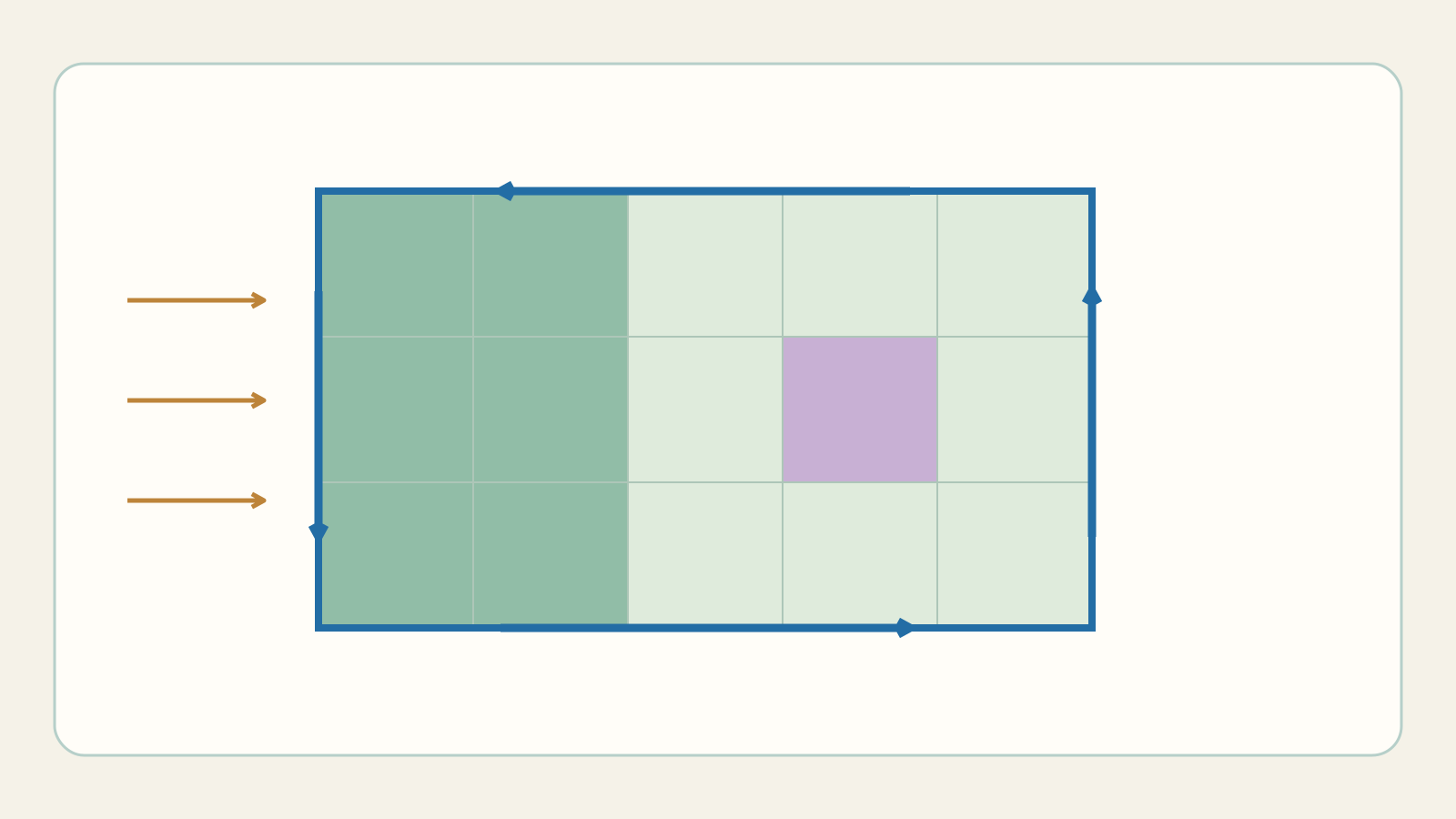
Previously we summed work along a path. Now close the path: can the same circulation be recovered from what happens inside? Green connects two different calculations, provided boundary and domain assumptions hold. Start with a rectangle before circles, annuli and flux.
Green: from boundary to region · Learning-path index
1. Two views of the same quantity
Circulation is the line integral of F=(P,Q) around a closed curve: ∮C Pdx+Qdy. The circle on the integral marks a return to the start. It is not boundary length or field magnitude: directed components and signs matter.
The theorem connects this boundary sum to a double integral. The interior function is not P+Q but Q_x−P_y, with subscripts denoting partial derivatives. It describes local circulation density, not automatically an immersed object’s angular velocity.
2. Assumptions before the formula
Classically D is a bounded planar region with a simple closed piecewise regular boundary. P and Q have continuous first derivatives on an open neighbourhood of the region and its boundary. Rectangle corners are allowed; an undefined interior point violates the assumptions. Multiple boundary components follow later.
Positive traversal keeps the region to the left, counterclockwise when there are no holes. Reversal changes the boundary integral’s sign, not the geometric double integral on D. The comparison then needs an explicit minus sign.
3. Write and read Green
B=∮[∂D,+] P dx+Q dy
I=∬D (Q_x−P_y)dA
B=I
B_(−∂D)=−I
∂D means boundary of D; + fixes positive orientation. dA is positive area, not a carrier of counterclockwise orientation. For F=(−y,x), P_y=−1 and Q_x=1, so Q_x−P_y=1−(−1)=2. Keep both minus signs.
4. One rectangle, four sides, two calculations
Take D=[0,a]×[0,b], a,b>0, F=(−y,x). From the origin follow bottom rightward, right upward, top leftward, left downward. Horizontal sides have dy=0; vertical sides dx=0.
B₁=∫₀ᵃ0 dx=0
B₂=∫₀ᵇa dy=ab
B₃=∫ₐ⁰(−b)dx=(−b)(−a)=ab
B₄=∫[b,0]0 dy=0
B=0+ab+ab+0=2ab
I=∫₀ᵃ∫₀ᵇ2 dy dx=2ab
a=2, b=1 → B=I=4
The top contribution is positive because both P and dx are negative. This prevents integrating every side forward without changing its tangent direction.
5. Why those derivatives appear
For a general field add the four rectangle sides. Pair horizontal sides, then vertical ones; turn differences of values into integrals of derivatives using the fundamental theorem. All steps use the stated regularity assumptions.
B=∫₀ᵃ[P(x,0)−P(x,b)]dx+∫₀ᵇ[Q(a,y)−Q(0,y)]dy
P(x,0)−P(x,b)=−∫₀ᵇP_y(x,y)dy
Q(a,y)−Q(0,y)=∫₀ᵃQ_x(x,y)dx
B=−∫₀ᵃ∫₀ᵇP_y dy dx+∫₀ᵇ∫₀ᵃQ_x dx dy
 =∬D (Q_x−P_y)dA
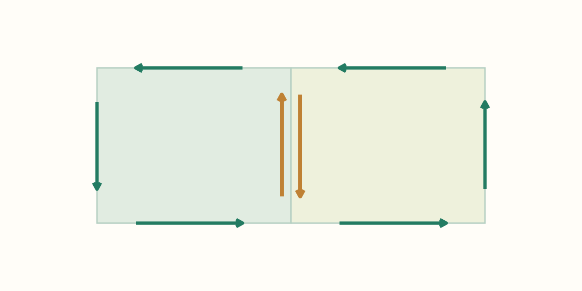
Joining adjacent cells traverses the shared edge twice in opposite directions, cancelling it and leaving the union’s boundary. This motivates general regions; the picture is not the technical limiting proof for curved domains.
6. Nonconstant interior density
For F=(−y³,x³) on the rectangle, P_y=−3y² and Q_x=3x². Density is 3x²+3y², not an arbitrary constant. Integrate in y, then x.
I=∫₀ᵃ∫₀ᵇ(3x²+3y²)dy dx
 =∫₀ᵃ[3x²y+y³]₀ᵇdx
 =∫₀ᵃ(3bx²+b³)dx
 =[bx³+b³x]₀ᵃ=ba³+ab³=ab(a²+b²)
B₂=a³b; B₃=ab³; B₁=B₄=0
a=2,b=1 → B=I=2(4+1)=10
The lab computes the two quadratures independently. Boundary calculation may already be exact while the interior sum still has error. A discrepancy shrinking with n does not refute the analytic identity.
7. The region need not be rectangular
Take triangle vertices (0,0),(a,0),(0,b) in this positive order. Its area is ab/2. For F=(−y,x), density 2 gives I=ab. The slanted side from (a,0) to (0,b) supplies all circulation; axis sides give zero.
r(t)=(a(1−t),bt), 0≤t≤1
r′=(−a,b), F(r)=(−bt,a(1−t))
F(r)·r′=abt+ab(1−t)=ab
B=∫₀¹ab dt=ab
I=∫[0,a]∫[0,b(1−x/a)]2dy dx=ab
The upper y bound depends on x and follows the hypotenuse. In the lab x=au, y=b(1−u)v maps a parameter square to the triangle. Its area weight is J=ab(1−u), not constant ab.
8. Compute area from a boundary
Choose P=−y/2, Q=x/2, giving Q_x−P_y=1. Green turns the integral of 1, area, into a boundary integral. For ellipse x=a cos t, y=b sin t, 0≤t≤2π, the integrand simplifies without square roots.
Area(D)=1/2 ∮[∂D,+](x dy−y dx)
−y x′/2+x y′/2=(ab/2)(sin²t+cos²t)=ab/2
Area(ellipse)=∫₀²πab/2 dt=πab
For a simple polygon, segment integration gives ½Σ(x_i y_(i+1)−x_(i+1)y_i), closing last vertex to first. For (0,0),(3,0),(0,2), (0+6+0)/2=3. Reversal gives −3, signed area; geometric area remains 3. Self-intersecting contours require different treatment.
9. Regions with holes: every boundary counts
Green extends to finitely many holes with piecewise regular boundaries when the field is C¹ near the entire closed region, holes excluded. Each component leaves D on the left: outer counterclockwise, hole boundaries clockwise. The outer loop alone is insufficient.
D={r≤√(x²+y²)≤R}, 0<r<R
∮outer,+F·dr + ∮inner,−F·dr = ∬D(Q_x−P_y)dA
F=(−y,x): B_outer=2πR²; B_inner=−2πr²
B=2π(R²−r²)=2 Area(D)
R=2,r=1 → 8π−2π=6π
Here + and − mark counterclockwise and clockwise circle traversal. A cut connecting the loops has opposite contributions on its two faces. Simple connectedness is unnecessary for this extended version, provided all boundary components and field assumptions are respected.
10. Why the angular field does not refute Green
F=(−y/(x²+y²),x/(x²+y²)) has Q_x−P_y=0 away from the origin. Every counterclockwise origin-centred circle has circulation 2π. Green cannot use its filled disk: the field is undefined at the interior origin. A grid missing that point does not repair the hypothesis.
D={ρ≤R}: (0,0)∈D; ∄F(0,0)
D={r≤ρ≤R}, r>0 → B_outer=2π, B_inner=−2π
B_total=0=∬D0 dA
On the annulus the origin is outside the region: the field is regular nearby and Green works with both loops. Omitting the inner loop leaves 2π, changing the contour rather than finding a theorem exception.
11. The second form: outward flux
For positive traversal the outward normal is to the tangent’s right, with n ds=(dy,−dx). Flux is ∮Pdy−Qdx. Apply circulation Green to the auxiliary field (−Q,P); interior density becomes P_x+Q_y.
∮[∂D,+] F·n ds=∮[∂D,+] Pdy−Qdx
 =∬D(P_x+Q_y)dA
F=(x,y): P_x+Q_y=1+1=2
D={x²+y²≤R²} → Flux_out=2πR²
In the lab reversal keeps the normal to the tangent’s right: it becomes inward and flux changes sign. Physical flux with a fixed outward normal does not change merely by reparametrising; the normal choice must also be preserved. Surface and volume versions come later.
12. Read the lab’s two sums
Left: midpoint contributions along each boundary component. Right: n² parameter cells mapped into the region with the Jacobian. The program does not derive one answer from the other using Green; the calculations are independent.
ΔB_i=[P(r(t_i*))x′(t_i*)+Q(r(t_i*))y′(t_i*)]Δt_i
ΔI_ij=(Q_x−P_y)(x_ij,y_ij) J(u_i*,v_j*) Δu Δv
D={ρ≤R}: ρ=Ru, θ=2πv → J=2πR²u
D={r≤ρ≤R}: ρ=r+(R−r)u → J=2πρ(R−r)
One boundary cell per step; interior strips progress proportionally. Partial sums need not agree because selected fragments are not the closed boundary of the same subregion. At completion compare B with sI, s=1 positive and −1 reversed. Inapplicable cases disable rather than force comparison.
13. A checklist before calculating
Is the contour simple and closed, or the correct boundary components around holes? Is the region on the left? Is the field C¹ inside and near the boundary? Did I compute Q_x−P_y, not P_x−Q_y? Did polar coordinates include area weight? Only then choose the easier integral.
Ten guided experiments distinguish a true identity, a failed assumption and numerical error. Sampled arrows and finite sums are not a general proof. Stage 27 will extend the language to parametric surfaces, area, normals and surface integrals.
Exercises: try before revealing
1. Find interior density for F=(−y,x) and F=(2x,2y).
Show the explained answer
First Q_x−P_y=1−(−1)=2. Second 0−0=0: a gradient, not an everywhere-zero field.
2. Rectangle 2×1, F=(−y,x): add four sides.
Show the explained answer
Bottom 0, right 2, top 2, left 0: B=4. Region calculation 2×Area=2×2=4. At the top P<0 and dx<0, making a positive contribution.
3. Reverse the rectangle boundary: do both B and I become negative?
Show the explained answer
No: B changes 4 to −4, I stays 4. Compare B=−I. Curve direction does not make geometric area negative.
4. F=(−y³,x³), rectangle 2×1: exact value?
Show the explained answer
Density 3x²+3y². I=ab(a²+b²)=2×1×(4+1)=10. Boundary right a³b=8 and top ab³=2, total 10.
5. Triangle (0,0),(3,0),(0,2), F=(−y,x): circulation?
Show the explained answer
Area=3×2/2=3; density 2, hence B=6. The oriented hypotenuse (3,0) to (0,2) supplies all of it.
6. Ellipse semi-axes 3,2 and F=(−y/2,x/2): what does B measure?
Show the explained answer
Q_x−P_y=1: positive-boundary B measures area πab=6π. A different field such as (−y,x) has density 2 and doubles circulation.
7. The vertex formula gives −3: is geometric area negative?
Show the explained answer
No: for a simple polygon the sign indicates orientation. Geometric area is |−3|=3. First check that the contour does not self-intersect.
8. Annulus R=2,r=1, F=(−y,x): both boundaries?
Show the explained answer
Outer counterclockwise 8π; inner clockwise −2π. Total 6π=2×π(4−1). Traversing both counterclockwise gives the wrong inner-boundary sign.
9. Angular field on annulus: why does 2π not contradict zero density?
Show the explained answer
2π is only the outer contribution. The complete boundary includes inner −2π: total zero. Omitting it no longer integrates over ∂D.
10. Angular field on a disk: may Green apply because the grid misses the origin?
Show the explained answer
No. The field is undefined at the region’s origin. Assumptions concern the whole region, not sampled points. Circle circulation 2π is valid; using the filled disk is not.
11. F=(x,y), disk R=2: outward flux and reversal?
Show the explained answer
Density P_x+Q_y=2, outward flux 8π. Reversed Pdy−Qdx uses the inward normal and gives −8π. With the outward normal fixed, physical flux remains 8π.
12. Polynomial rectangle: B=10, I≈9.84375 at n=4. Contradiction?
Show the explained answer
No: both analytic references are 10. The interior midpoint rule still has error 0.15625. Increasing n shrinks it. Green does not promise exact equality of different finite quadratures.
Before: line integrals, work and potential · Learning-path index